
- Intro
- Load library
- Load data
- Data exploration
- Data transformation
- Combine test and train for feature selection
- Recode survive for caret train as 1 and 0 are not valid level name in R
- Extract Title
- Remove those title different from Miss, Master, Mr and Mrs since they are low frequency
- Make Missingage predictor before we impute Age
- Use Title to predict Age
- Impute Embarked by median
- Impute Fare by mean
- Family name
- Transform Fare to log(Fare)
- Make groupsize predictor
- Final look
- Training
- Evaluation
- Using other set of predictors
- Using other set of predictors
- Using another set of predictions
- Make other predictor
- Summary
Intro
This is the analysis I used to create the prediction for Kaggle competition. The purpose of the analysis is to use machine learning to predict the survival probability of people on the Titanic. The dataset is provided as follow:
Dataset is divided into train and test set.
Passenger’s information such as Name, Age, Pclass, etc. is provided in both train and test set
The outcome (survival) indicates whether that passenger has survived or perished. This only presents in the training set.
There are some missing value in both data set
By using different machine learning algorithm, predictions can be made for people on the test dataset. In this project, I used a variaty of methods, some are just blackbox, some can be visualized fully or partially.
Load library
library(tidyverse)
library(doParallel)
library(caret)
library(lubridate)
library(patchwork)
library(caretEnsemble)
library(pROC)
library(partykit)
Load data
train0 <- read_csv("./titanic/train.csv",
                   col_types = cols(
                     Survived = col_factor(ordered = FALSE, include_na = T),
                     Pclass = col_factor(),
                     Sex = col_factor(),
                     Embarked = col_factor()
                   ))
intrain <- dim(train0)[1]
test0 <- read_csv("./titanic/test.csv",
                  col_types = cols(
                    Pclass = col_factor(),
                    Sex = col_factor(),
                    Embarked = col_factor()
                  ))
Data exploration
First glimpse at our data
glimpse(train0)## Observations: 891
## Variables: 12
## $ PassengerId <dbl> 1, 2, 3, 4, 5, 6, 7, 8, 9, 10, 11, 12, 13, 14, 15,...
## $ Survived <fct> 0, 1, 1, 1, 0, 0, 0, 0, 1, 1, 1, 1, 0, 0, 0, 1, 0,...
## $ Pclass <fct> 3, 1, 3, 1, 3, 3, 1, 3, 3, 2, 3, 1, 3, 3, 3, 2, 3,...
## $ Name <chr> "Braund, Mr. Owen Harris", "Cumings, Mrs. John Bra...
## $ Sex <fct> male, female, female, female, male, male, male, ma...
## $ Age <dbl> 22, 38, 26, 35, 35, NA, 54, 2, 27, 14, 4, 58, 20, ...
## $ SibSp <dbl> 1, 1, 0, 1, 0, 0, 0, 3, 0, 1, 1, 0, 0, 1, 0, 0, 4,...
## $ Parch <dbl> 0, 0, 0, 0, 0, 0, 0, 1, 2, 0, 1, 0, 0, 5, 0, 0, 1,...
## $ Ticket <chr> "A/5 21171", "PC 17599", "STON/O2. 3101282", "1138...
## $ Fare <dbl> 7.2500, 71.2833, 7.9250, 53.1000, 8.0500, 8.4583, ...
## $ Cabin <chr> NA, "C85", NA, "C123", NA, NA, "E46", NA, NA, NA, ...
## $ Embarked <fct> S, C, S, S, S, Q, S, S, S, C, S, S, S, S, S, S, Q,...We can see that: - PassengerID is just a sequence of number to distinguish passengers, hence it has no predictive power.
Name follows a pattern with Familyname, Title and Firstname, it shows a potential to extract those components
SibSp and Parch: aren’t those in the same family have the same familyname? Possibly have a relationship with family name
Ticket does not follow any obvious pattern
A lot of missing values in Cabin
Dealing with NA
How many NA values?
- in train set
train0 %>% map_df(~sum(is.na(.)))## # A tibble: 1 x 12
## PassengerId Survived Pclass Name Sex Age SibSp Parch Ticket Fare
## <int> <int> <int> <int> <int> <int> <int> <int> <int> <int>
## 1 0 0 0 0 0 177 0 0 0 0
## # ... with 2 more variables: Cabin <int>, Embarked <int>- in test set
test0 %>% map_df(~sum(is.na(.)))## # A tibble: 1 x 11
## PassengerId Pclass Name Sex Age SibSp Parch Ticket Fare Cabin
## <int> <int> <int> <int> <int> <int> <int> <int> <int> <int>
## 1 0 0 0 0 86 0 0 0 1 327
## # ... with 1 more variable: Embarked <int>Dealing with NA:
Remove Cabin as there are too much NA
Using median for Fare, only 1 value is missing
Using the highest frequency value for Embarked
The only predictor relating to Age is Name (Title e.g Mr, Miss, etc), so missing Age is replace by the mean of Age of people with the same title.
Other methods like knnImpute or BagImpute or even some models which can handle NA values can be used to impute. However, those seems unnecessary complicated methods since they consider all other predictors to find NA values, We certainly know that only some predictors are directly relating predictors with missing NA.
Visualization
Fare
p1 <- train0 %>% ggplot() + geom_histogram(aes(Fare, fill = Survived)) + labs(title = "Histogram of Fare \nin relation with Survived")
p2<- train0 %>% ggplot() + geom_histogram(aes(Fare, fill = Survived), position = "fill") + labs(title = "Percentage of Fare \nin relation with Survived")
p1 + p2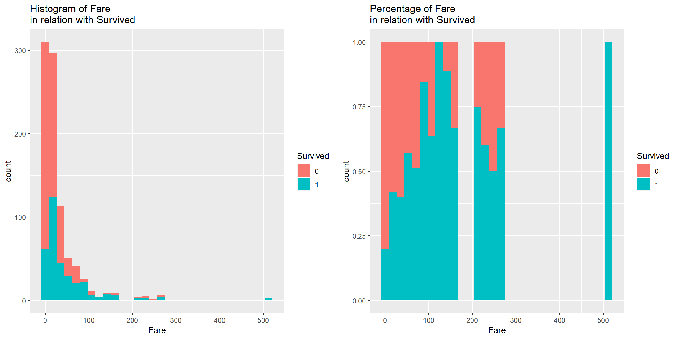
Distibution of Fare is skewed to the right, transform it with log10 to normalize
p1 <- train0 %>% ggplot() + geom_histogram(aes(log10(Fare+1), fill = Survived)) + labs(title = "Histogram of Fare \nin relation with Survived")
p2<- train0 %>% ggplot() + geom_histogram(aes(log10(Fare+1), fill = Survived), position = "fill") + labs(title = "Percentage of Fare \nin relation with Survived")
p1 + p2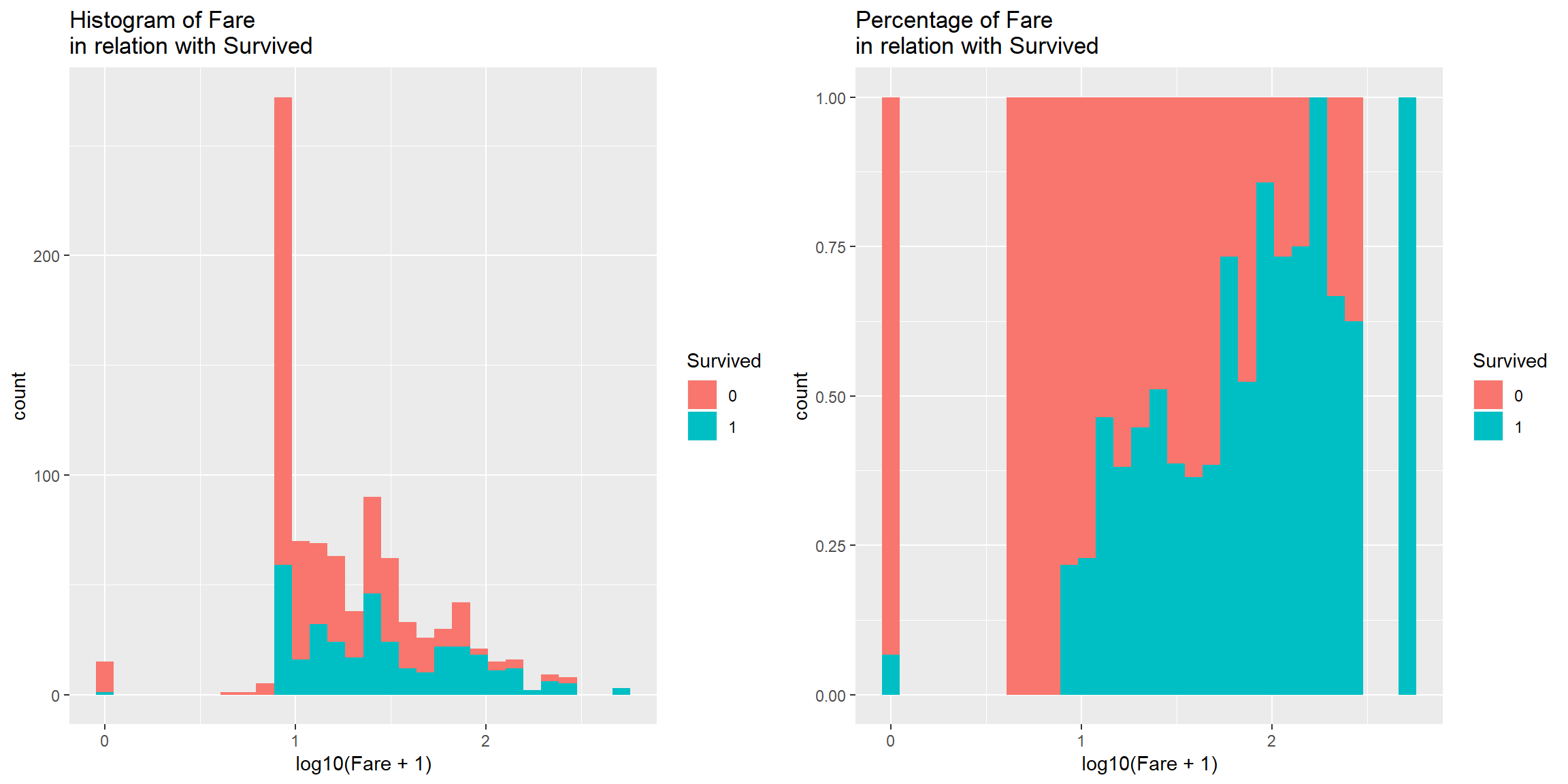
There is a patern in Fare in relation with Survived. More expensive ticket, higher chance to Survive (to an extend).
Good predictor
Pclass
train0 %>% ggplot() + geom_bar(aes(fct_relevel(Pclass, "1", "2"), fill = Survived)) + scale_x_discrete(name = "Pclass")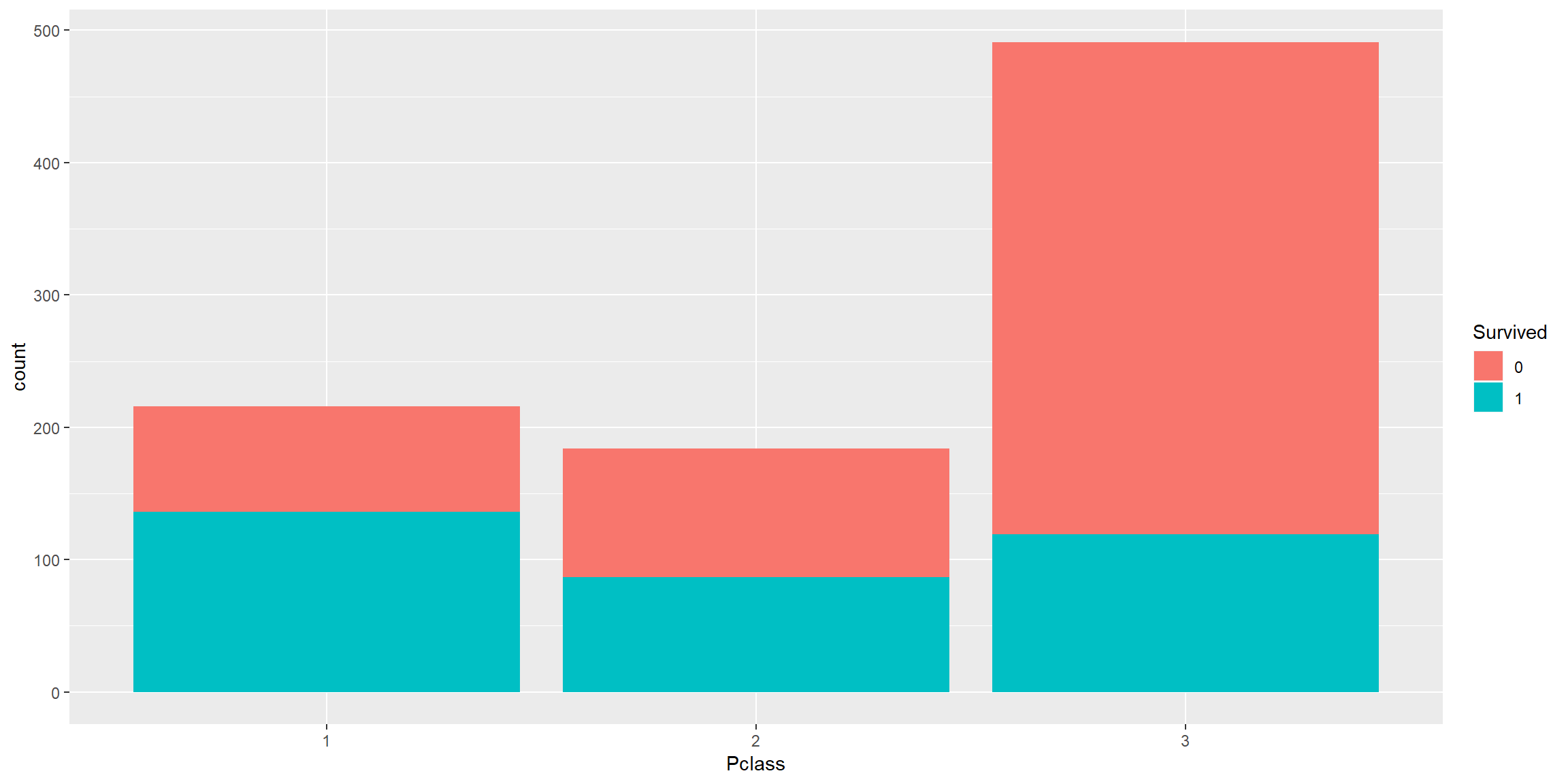
Pclass 1 > Pclass 2 > Pclass 3 in survival rate and there are much more people in Pclass 3 than Pclass 1 and 2.
train0 %>% ggplot() + geom_boxplot(aes(fct_reorder(Pclass,Fare), Fare)) + scale_x_discrete(name = "Pclass")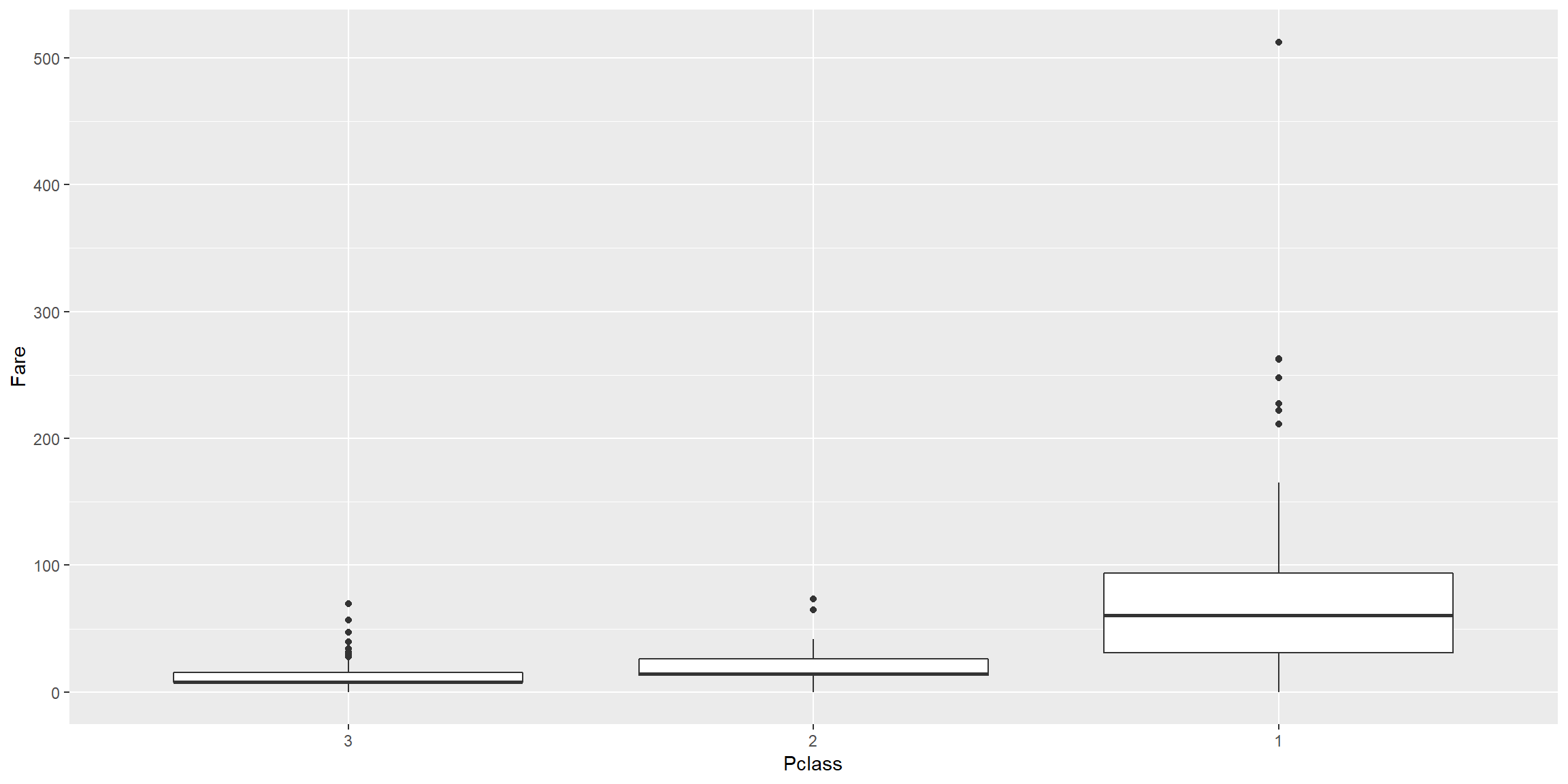
The cost of Ticket increases from PClass 3 (cheapest) to Pclass 1 (most expensive).
This makes sense as the upper class who stayed in Pclass 1 would have more money hence have better chance to survive.
Good predictor
Sex
train0 %>% ggplot() + geom_bar(aes(Sex, fill = Survived))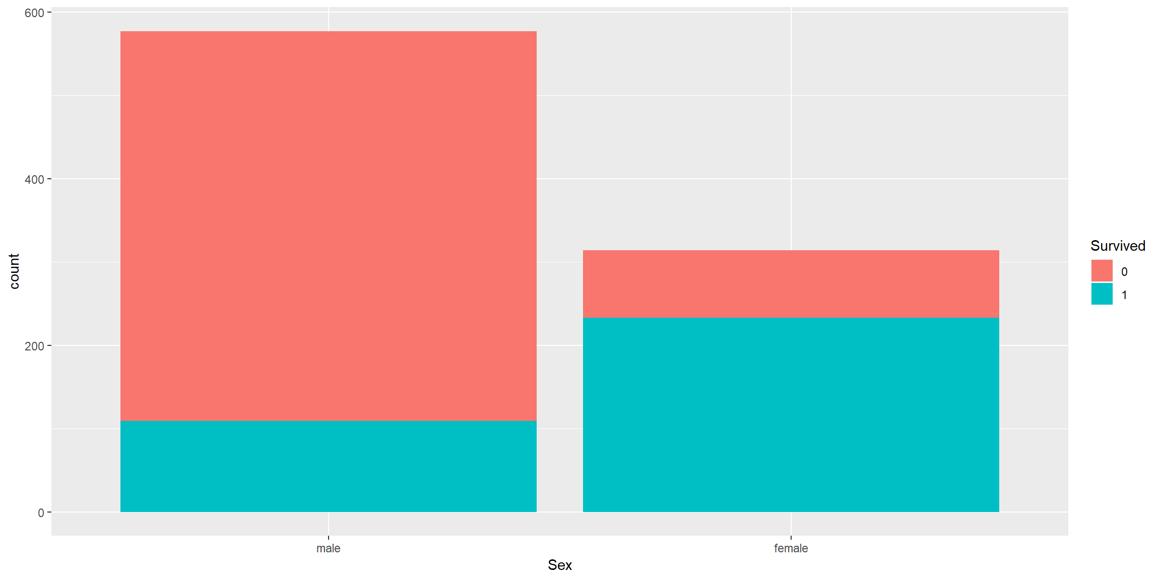
Female have better survival rate as women and children are usually being rescued first.
Good predictor
Data transformation
Combine test and train for feature selection
combined <- bind_rows(train0, test0)Recode survive for caret train as 1 and 0 are not valid level name in R
combined$Survived <- fct_recode(combined$Survived, "Lived" = "1", "Died" = "0") %>%
  fct_relevel("Lived")
Extract Title
combined <- combined %>% mutate(Title = str_extract(Name, ", (\\w)+")) %>%
  mutate(Title = str_extract(Title, "\\w+"))
Remove those title different from Miss, Master, Mr and Mrs since they are low frequency
combined %>% ggplot() + geom_bar(aes(Title))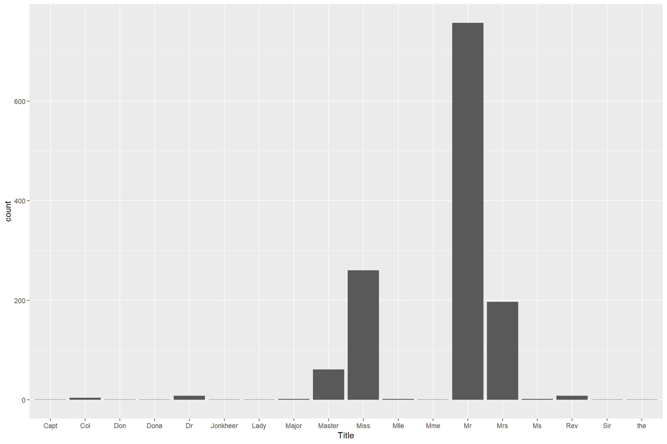
Then combine them into Others
combined <- combined %>%
  mutate(Title = ifelse(Title %in% c("Miss", "Master", "Mr", "Mrs"), Title,"Others"))
How this Title predictor look
combined[1:intrain,] %>% ggplot() + geom_bar(aes(Title, fill = fct_relevel(Survived, "Died"))) + labs(fill = "Survived")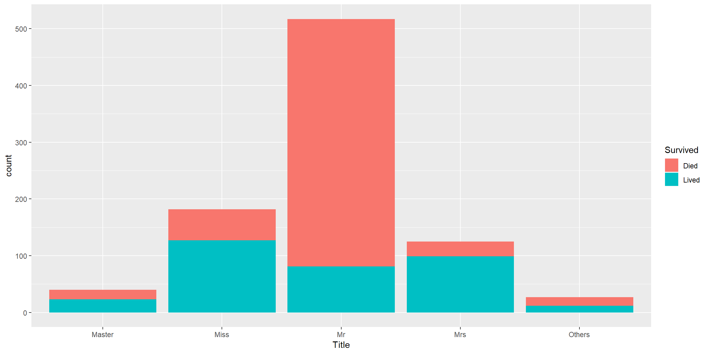 Good predictor.
In combination with Pclass, we can see a more detail picture.
combined[1:intrain,] %>%
    group_by(Title, Pclass, Survived) %>%
    summarise(each = n()) %>% ungroup() %>% group_by(Title, Pclass) %>% mutate(Tot = sum(each)) %>%
  mutate(Survivalrate = each/Tot) %>%
  ungroup() %>% filter(Survived == "Lived") %>%
  ggplot() + geom_tile(aes(fct_relevel(Pclass,"1","2"), fct_relevel(Title,"Master", "Miss", "Mrs", "Mr"), fill = Survivalrate)) + scale_fill_viridis_c() + xlab("Pclass") + ylab("Title")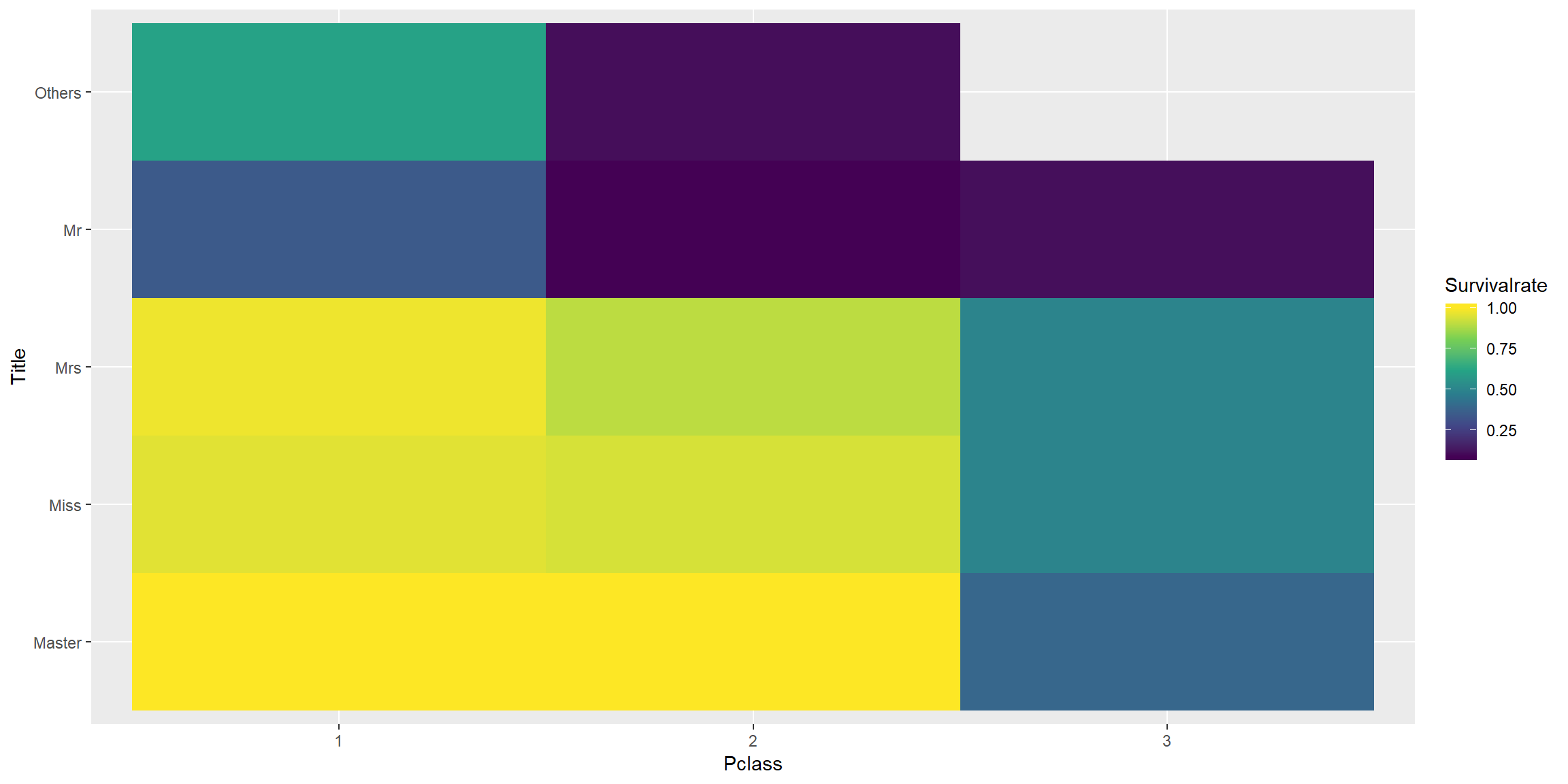
Make Missingage predictor before we impute Age
combined <- combined %>% mutate(MissingAge = is.na(Age))Use Title to predict Age
Master are underage male children(Fact). Take mean Age from train set and use it to replace NA from all data with Master title
meanMasterAge <- combined %>%
  slice(1:dim(train0)[1]) %>%
  filter(Title == "Master") %>%
  summarise(mean(Age, na.rm = T)) %>%
  pull()
combined <- combined %>%
  mutate(Age = ifelse(Title == "Master" & is.na(Age), meanMasterAge ,Age ))
Impute Age based on other Title
combined[is.na(combined$Age) & combined$Title == "Mr",]$Age <- mean(combined[1:intrain,][combined[1:intrain,]$Title == "Mr",]$Age, na.rm = T)
combined[is.na(combined$Age) & combined$Title == "Miss",]$Age <- mean(combined[1:intrain,][combined[1:intrain,]$Title == "Miss",]$Age, na.rm = T)
combined[is.na(combined$Age) & combined$Title == "Mrs",]$Age <- mean(combined[1:intrain,][combined[1:intrain,]$Title == "Mrs",]$Age, na.rm = T)
combined[is.na(combined$Age) & combined$Title == "Others",]$Age <- mean(combined[1:intrain,][combined[1:intrain,]$Title == "Others",]$Age, na.rm = T)
Impute Embarked by median
combined[is.na(combined$Embarked),]$Embarked <- "S"Impute Fare by mean
combined[is.na(combined$Fare),]$Fare <- mean(combined[1:intrain,][combined[1:intrain,]$Pclass == 3,]$Fare, na.rm = T)Family name
combined <- combined %>% mutate(Familyname = str_extract(Name, "^.+,")) %>%
  mutate(Familyname = str_sub(Familyname,1, -2))
Transform Fare to log(Fare)
combined <- combined %>% mutate(Fare = log10(Fare +1))Make groupsize predictor
A. There are people with same Ticket but different Family name B. There are people with same Familyname but different Ticket C. There are people with same Familyname and same Ticket
The groupsize of a person is determined by number of other people with same ticket and family name. (A + B - C)
combined <- combined %>% group_by(Ticket, Familyname) %>% mutate(nAll = n()) %>%
  ungroup() %>% group_by(Ticket) %>% mutate(nTicket = n()) %>%
  ungroup() %>% group_by(Familyname) %>% mutate(nFamilyname = n()) %>%
  ungroup() %>% mutate(Groupsize = nTicket + nFamilyname - nAll)

combined <- combined %>% select(-nTicket, -nFamilyname)
How this new groupsize predictor look
combined[1:intrain,] %>%
  ggplot() + geom_bar(aes(Groupsize, fill = fct_relevel(Survived, "Died")), position = "fill")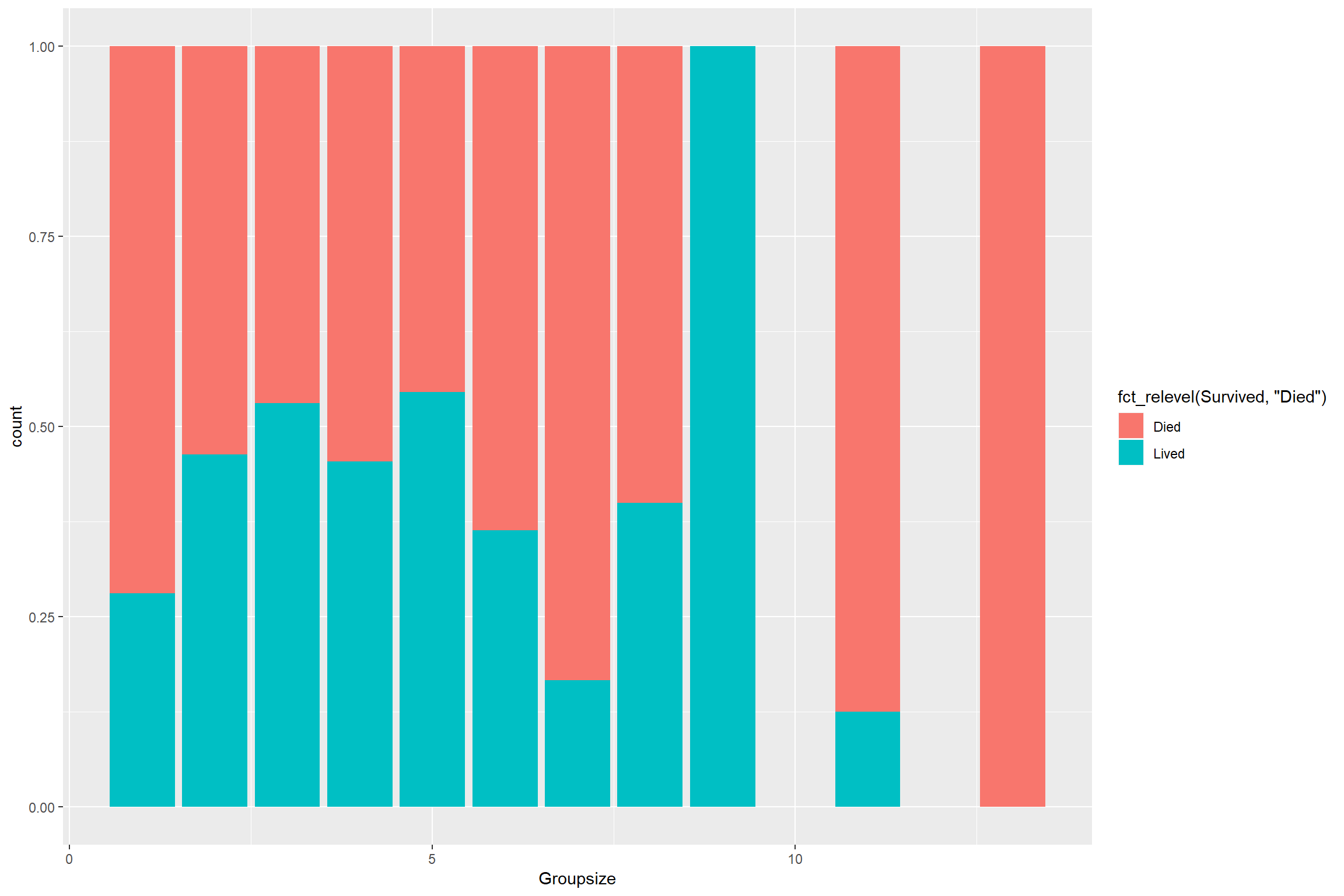
combined[1:intrain,] %>%
group_by(Pclass,Groupsize, Title, Survived) %>%
summarise(each = n()) %>% ungroup() %>% group_by(Pclass, Groupsize, Title) %>% mutate(Tot = sum(each)) %>%
mutate(Survivalrate = each/Tot) %>%
ungroup() %>% filter(Survived == "Lived") %>%
ggplot() + geom_tile(aes(fct_relevel(Title, "Master", "Miss", "Mrs"), Groupsize, fill = Survivalrate)) + scale_fill_viridis_c() + xlab("Title") + ylab("Groupsize") + facet_wrap(.~fct_relevel(Pclass, "1", "2"))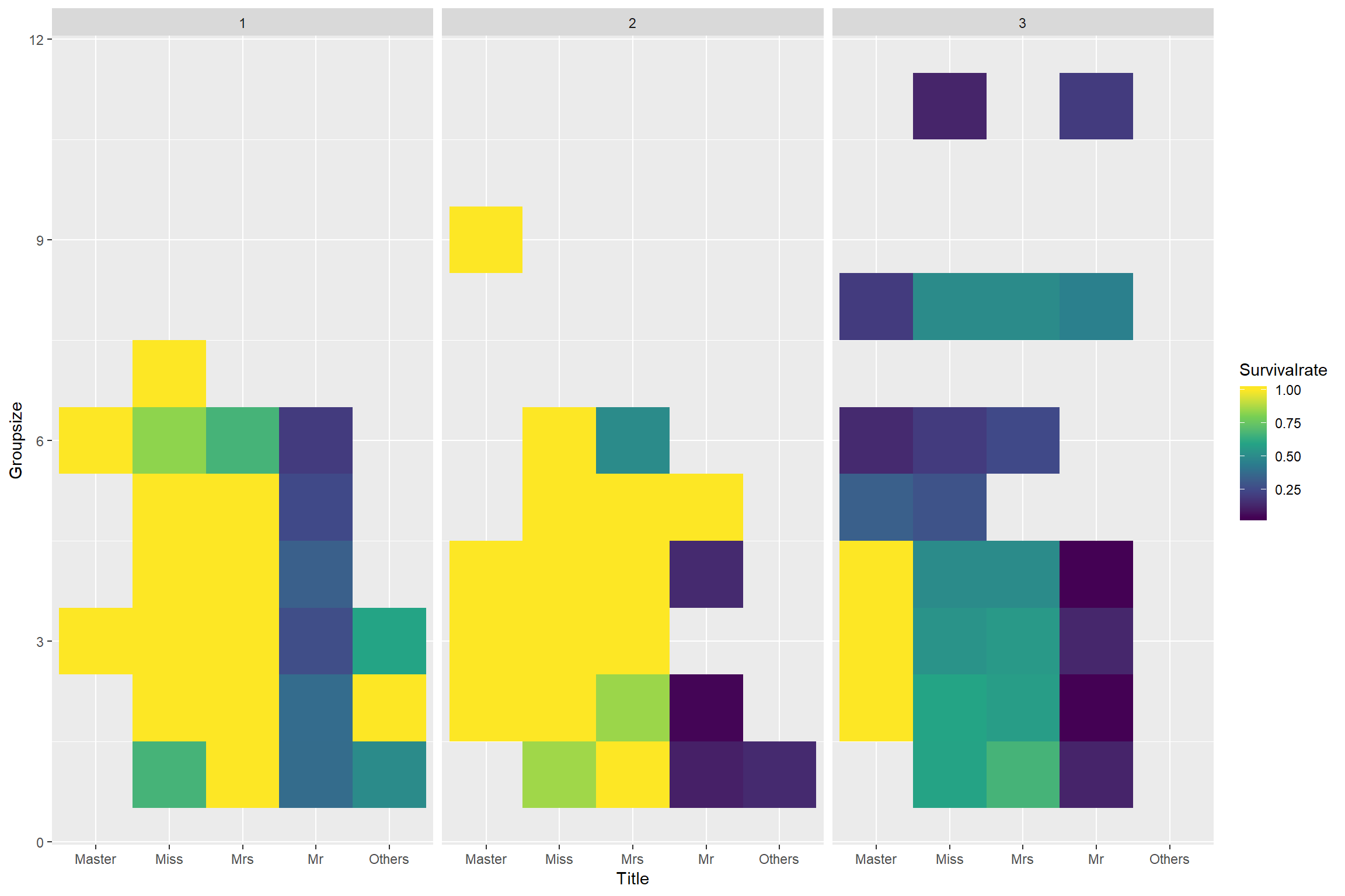 Some pattern but not really clear.
Final look
glimpse(combined)## Observations: 1,309
## Variables: 17
## $ PassengerId <dbl> 1, 2, 3, 4, 5, 6, 7, 8, 9, 10, 11, 12, 13, 14, 15,...
## $ Survived <fct> Died, Lived, Lived, Lived, Died, Died, Died, Died,...
## $ Pclass <fct> 3, 1, 3, 1, 3, 3, 1, 3, 3, 2, 3, 1, 3, 3, 3, 2, 3,...
## $ Name <chr> "Braund, Mr. Owen Harris", "Cumings, Mrs. John Bra...
## $ Sex <fct> male, female, female, female, male, male, male, ma...
## $ Age <dbl> 22.00000, 38.00000, 26.00000, 35.00000, 35.00000, ...
## $ SibSp <dbl> 1, 1, 0, 1, 0, 0, 0, 3, 0, 1, 1, 0, 0, 1, 0, 0, 4,...
## $ Parch <dbl> 0, 0, 0, 0, 0, 0, 0, 1, 2, 0, 1, 0, 0, 5, 0, 0, 1,...
## $ Ticket <chr> "A/5 21171", "PC 17599", "STON/O2. 3101282", "1138...
## $ Fare <dbl> 0.9164539, 1.8590380, 0.9506082, 1.7331973, 0.9566...
## $ Cabin <chr> NA, "C85", NA, "C123", NA, NA, "E46", NA, NA, NA, ...
## $ Embarked <fct> S, C, S, S, S, Q, S, S, S, C, S, S, S, S, S, S, Q,...
## $ Title <chr> "Mr", "Mrs", "Miss", "Mrs", "Mr", "Mr", "Mr", "Mas...
## $ MissingAge <lgl> FALSE, FALSE, FALSE, FALSE, FALSE, TRUE, FALSE, FA...
## $ Familyname <chr> "Braund", "Cumings", "Heikkinen", "Futrelle", "All...
## $ nAll <int> 1, 2, 1, 2, 1, 1, 1, 5, 3, 2, 3, 1, 1, 7, 1, 1, 6,...
## $ Groupsize <int> 2, 2, 1, 2, 2, 3, 3, 5, 6, 2, 3, 2, 1, 11, 1, 1, 6...Training
Separate train and test set since we are done with Data transformation
Separate 20% of the train set into holdout set to evaluate the models, it is more convenient than using using upload test set to Kaggle everytime.
set.seed(12345)
notinholdout <- createDataPartition(train0$Survived, p = 0.8, list = F)

alltrain <- combined[1:intrain, ]

train <- combined[1:intrain, ] %>% slice(notinholdout)
holdout <- combined[1:intrain, ] %>% slice(-notinholdout)

test <- combined[-(1:intrain), ]
Validation folds
5 times repeated 10 folds is used to evaluate model’s parameters. It is usually specified inside the trainControl but separate this step is a requirement for caretEnsemble to make sure all folds are consistent for ensemble.
index <- createMultiFolds(train$Survived, k = 10, times = 5)Traincontrol
The index will take over other parameters, supply them just to get the labels right. We will use the metric ROC for this, so twoClassSummary and classProbs must be specified
trCtr_grid <- trainControl(method = "repeatedcv", repeats = 5,
                           number = 5,
                           index = index, savePredictions = "final", summaryFunction = twoClassSummary,
                           search = "grid", # By default
                           verboseIter=TRUE, classProbs = T)

trCtr_none <- trainControl(method = "none", classProbs = T)
= ## Setup parallel computing
cl <- makeCluster(7)
registerDoParallel(cl)
Get model info if needed
getModelInfo()$xgbTree$parameters## parameter class label
## 1 nrounds numeric # Boosting Iterations
## 2 max_depth numeric Max Tree Depth
## 3 eta numeric Shrinkage
## 4 gamma numeric Minimum Loss Reduction
## 5 colsample_bytree numeric Subsample Ratio of Columns
## 6 min_child_weight numeric Minimum Sum of Instance Weight
## 7 subsample numeric Subsample PercentageChoose Hyperparameters
C5.0grid <- expand.grid(.trials = c(1:9, (1:10)*10),
                       .model = c("tree", "rules"),
                       .winnow = c(TRUE, FALSE))

SVMgrid <- expand.grid(sigma = c(0, 0.01, 0.04, 0.2),
                       C= c(seq(0,1,0.2),10,500))

XGBgrid <- expand.grid(nrounds = 100, # Fixed. depend on datasize
                       max_depth = 6, # More will make model more complex and more likely to overfit. Choose only this due to computational barrier
                       eta = c(0.01,0.05, 0.1), # NEED FINE TUNE
                       gamma = 0, # it is usually OK to leave at 0
                       min_child_weight = c(1,2,3), # The higher value, the more conservative model is, NEED FINE TUNE
                       colsample_bytree = c(.4, .7, 1), # subsample by columns
                       subsample = 1) # subsample by row leave at 1 since we doing k-fold

rpartgrid <- expand.grid(cp = runif(30,0,0.5))

rfgrid <- expand.grid(mtry = 1:8)
Train models
Choose predictors
formula <- as.formula(Survived ~ Pclass + Sex + Title +
                        Age + MissingAge + SibSp + Parch + Groupsize +
                        Fare + Embarked)
We will use caret ensemble for easy training
set.seed(67659)

modelList <- caretList(
  formula, data = train,
  trControl=trCtr_grid,
  metric = "ROC",
  tuneList=list(
    rf=caretModelSpec(method="rf", tuneGrid= rfgrid),
    SVM=caretModelSpec(method="svmRadial", tuneGrid = SVMgrid,
                       preProcess = c("scale", "center")),
    xgb=caretModelSpec(method="xgbTree", tuneGrid = XGBgrid),
    rpart= caretModelSpec(method = "rpart", tuneGrid = rpartgrid),
    C5.0 = caretModelSpec(method = "C5.0", tuneGrid = C5.0grid)
    )
)
## Aggregating results
## Selecting tuning parameters
## Fitting mtry = 6 on full training set## Warning in nominalTrainWorkflow(x = x, y = y, wts = weights, info =
## trainInfo, : There were missing values in resampled performance measures.## Aggregating results
## Selecting tuning parameters
## Fitting sigma = 0.2, C = 0.4 on full training set
## Aggregating results
## Selecting tuning parameters
## Fitting nrounds = 100, max_depth = 6, eta = 0.05, gamma = 0, colsample_bytree = 0.4, min_child_weight = 2, subsample = 1 on full training set
## Aggregating results
## Selecting tuning parameters
## Fitting cp = 0.0228 on full training set
## Aggregating results
## Selecting tuning parameters
## Fitting trials = 100, model = rules, winnow = FALSE on full training setEvaluation
Evaluate in train data
dotplot(resamples(modelList))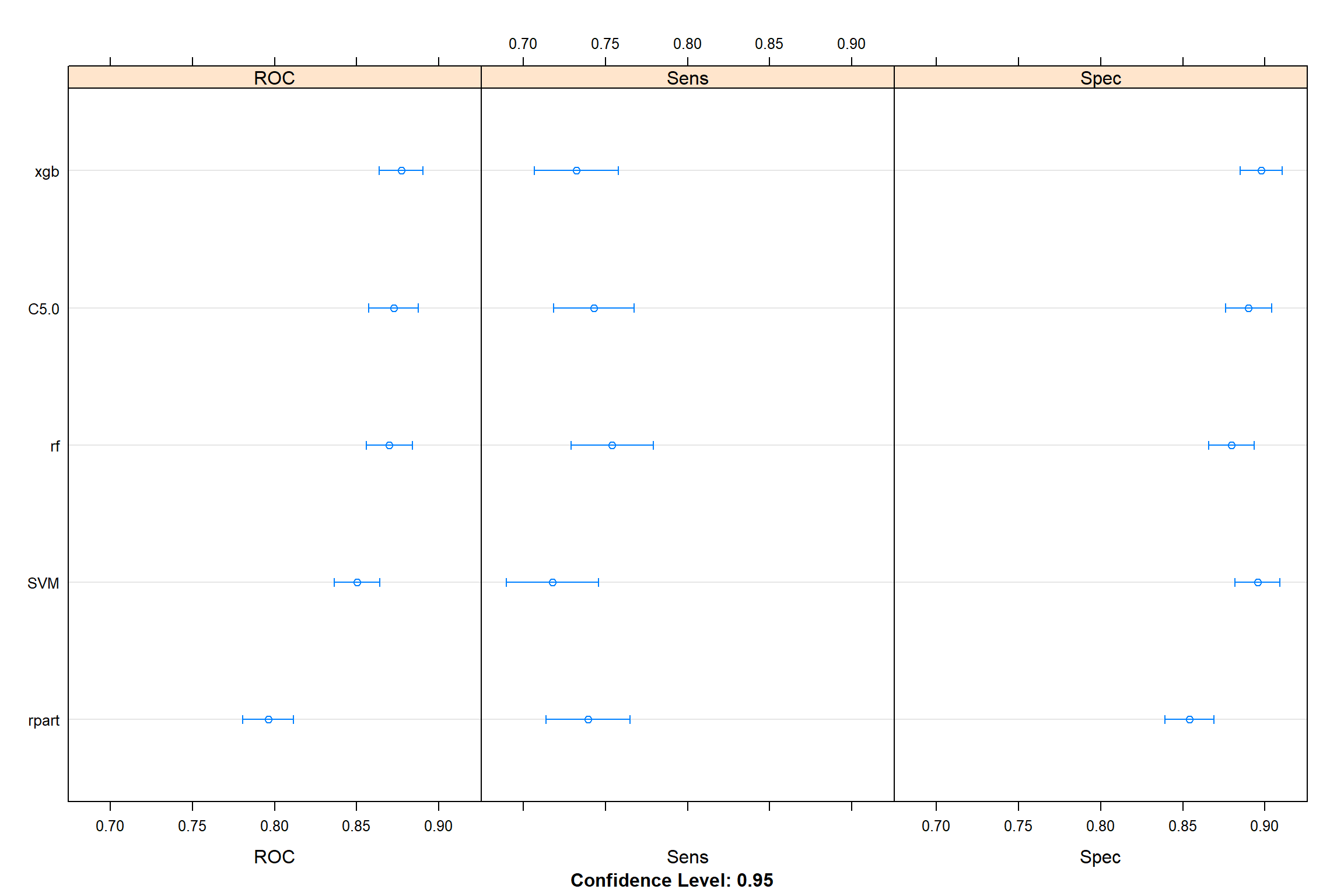
- rpart seems to be the worst model.
Let’s see if there is any significant different between them
diff(resamples(modelList), metric = "ROC") %>% summary()##
## Call:
## summary.diff.resamples(object = .)
##
## p-value adjustment: bonferroni
## Upper diagonal: estimates of the difference
## Lower diagonal: p-value for H0: difference = 0
##
## ROC
## rf SVM xgb rpart C5.0
## rf 0.019479 -0.007292 0.073719 -0.002654
## SVM 8.044e-05 -0.026771 0.054240 -0.022133
## xgb 0.01167 6.282e-07 0.081011 0.004639
## rpart < 2.2e-16 2.825e-11 < 2.2e-16 -0.076373
## C5.0 1.00000 4.563e-05 1.00000 < 2.2e-16- from here we can see that rpart and SVM are actually worse than the rest of models.
Any correlation between models
modelCor(resamples(modelList))## rf SVM xgb rpart C5.0
## rf 1.0000000 0.8413727 0.9532823 0.7763147 0.9494574
## SVM 0.8413727 1.0000000 0.8049344 0.6800322 0.8247340
## xgb 0.9532823 0.8049344 1.0000000 0.7609024 0.9228143
## rpart 0.7763147 0.6800322 0.7609024 1.0000000 0.7549545
## C5.0 0.9494574 0.8247340 0.9228143 0.7549545 1.0000000- all model are all correlated, which might not results in any improvement when trying to ensemble models. This is not unexpected as those model are quite strong. So we will not use any ensemble for now.
Let’s have a look at Importance of predictors in tree-based model
ggplot(varImp(modelList$rf)) + labs(title = "Random Forest") +
ggplot(varImp(modelList$C5.0)) + labs(title = "C5.0") +
ggplot(varImp(modelList$xgb)) + labs(title = "XGB") +
ggplot(varImp(modelList$rpart)) + labs(title = "rpart")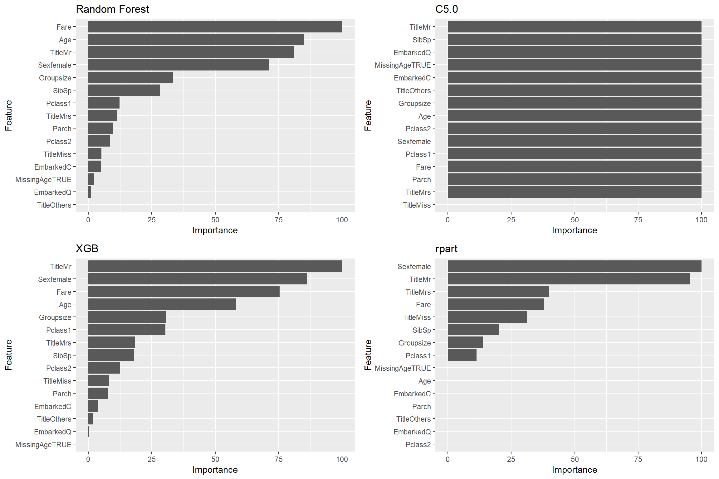
MissingAge predictors does not seem to do well across most models, in contrast, Groupsize perform really well.
Let’s visualize a tree in rpart model
plot(as.party(modelList$rpart$finalModel))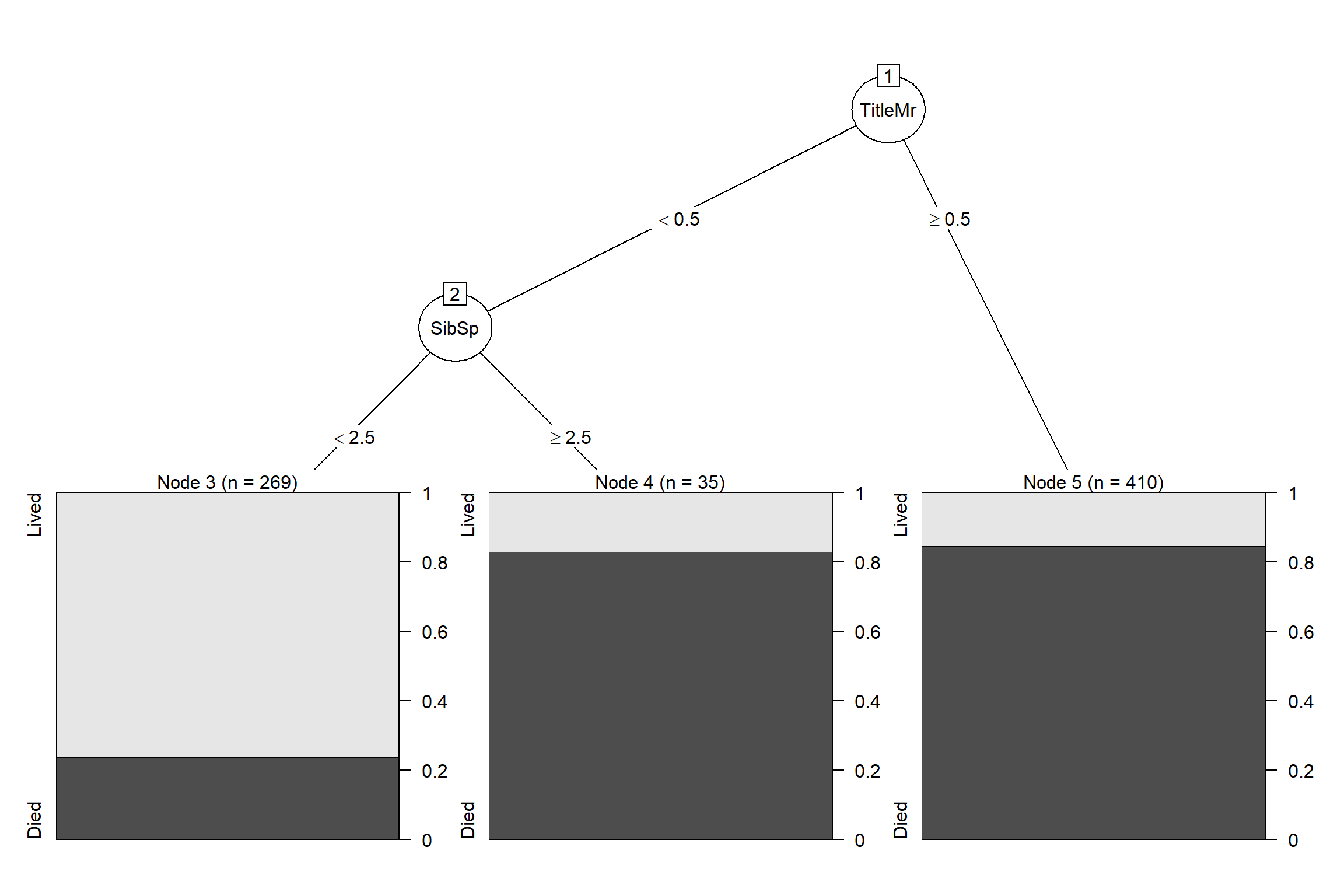
What a simple tree that can achieve almost 80% accuracy on unseen data (next part)
Evaluate in holdout data
Accuracy check:
map(modelList, ~predict(., newdata = holdout)) %>%
  map( ~ confusionMatrix(holdout$Survived, .)) %>%
  map_df(~.$overall["Accuracy"])
## # A tibble: 1 x 5
## rf SVM xgb rpart C5.0
## <dbl> <dbl> <dbl> <dbl> <dbl>
## 1 0.808 0.825 0.819 0.797 0.825ROC and AUC
modROC <- map(modelList, ~predict(. , newdata = holdout, type = "prob")) %>%
  map(~roc(predictor = .x$Lived,
           response = holdout$Survived,
           levels = rev(levels(holdout$Survived)),
           print.auc = TRUE)
)

aucROC <- modROC %>% map_df(~.$auc) %>% gather(key = "model", value = "ROC") %>%
  arrange(desc(ROC)) %>%
  mutate(ROC = round(ROC, digits = 3)) %>% unite("auc", model, ROC, sep = "'s AUC: ") %>%
  pull() %>% str_c(collapse = "\n")

ggroc(modROC) + geom_text(aes(x = 0.5, y = 0.5, label = aucROC), color = "black") + scale_color_discrete(name = "Model")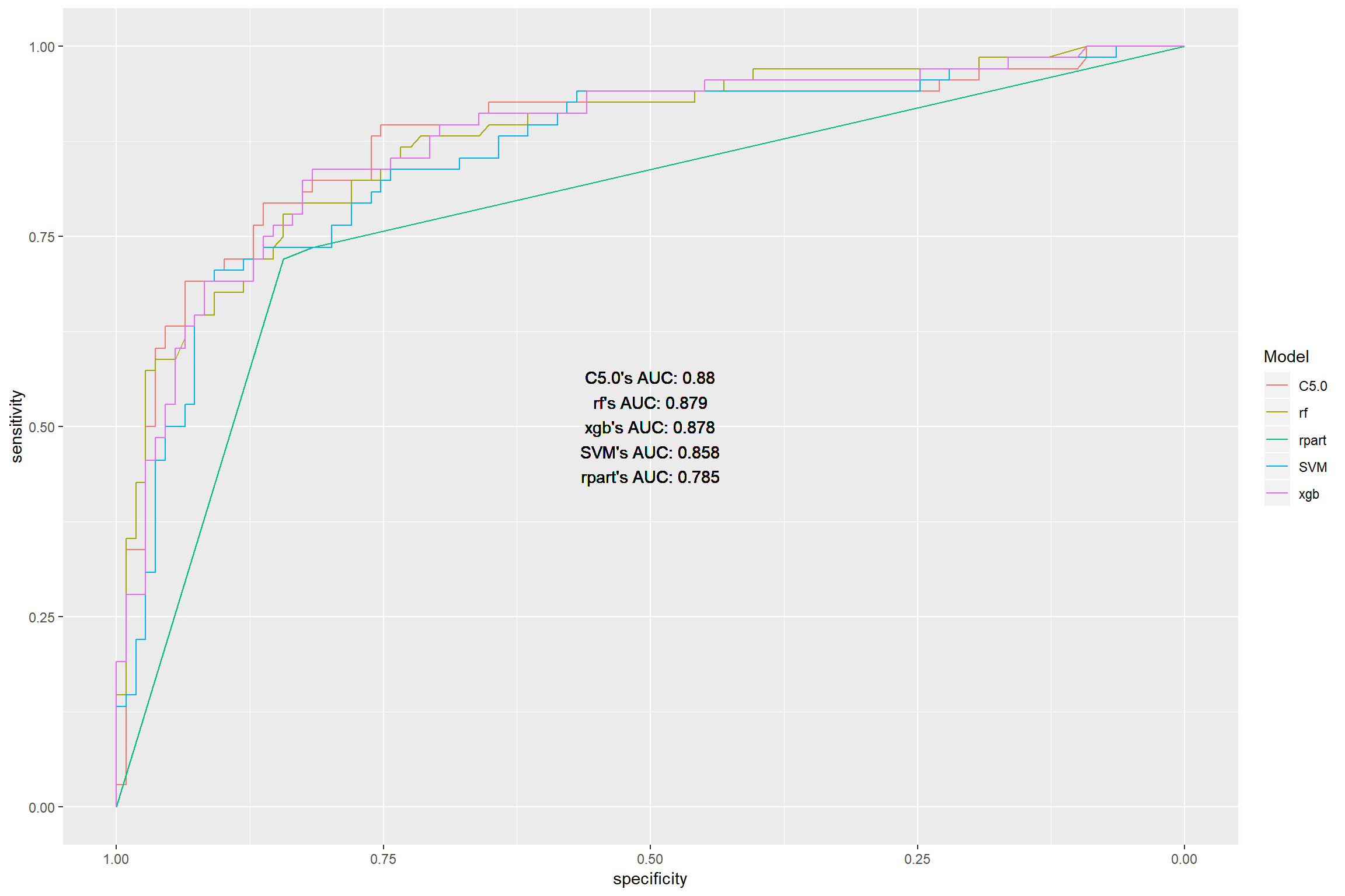
Ranking on best performance:
C5.0
Random Forest
- Extreme gradient boosting
Supportive vector machines
Decision tree
Evaluate on test data
Extract best tunes from models then train them again using all training data with no resampling method. After that, predict data on test data and print csv out to put on kaggle
set.seed(6759)

rf_f <- train(formula, data = alltrain, trControl = trCtr_none, method = "rf",
              tuneGrid = modelList$rf$bestTune)

SVM_f <- train(formula, data = alltrain, trControl = trCtr_none, method = "svmRadial",
               tuneGrid = modelList$SVM$bestTune, preProcess = c("scale", "center"))

xgb_f <- train(formula, data = alltrain, trControl = trCtr_none, method = "xgbTree",
               tuneGrid = modelList$xgb$bestTune)

rpart_f <- train(formula, data = alltrain, trControl = trCtr_none, method = "rpart",
                 tuneGrid = modelList$rpart$bestTune)

C5.0_f <- train(formula, data = alltrain, trControl = trCtr_none, method = "C5.0",
                tuneGrid = modelList$C5.0$bestTune)

all <- list(rf = rf_f, SVM = SVM_f, xgb = xgb_f, rpart = rpart_f, C5.0 = C5.0_f)

finaltest <- predict(all, newdata = test, na.action = na.pass)

prefix <- "all_ROC"

for (i in names(finaltest)){
  bind_cols(PassengerID = test0$PassengerId, Survived = finaltest[[i]]) %>%
    mutate(Survived = fct_recode(Survived, "1" = "Lived", "0" = "Died")) %>%
    write_csv(str_c("./prediction/", prefix,"_" ,i,"_", today(), ".csv"))
}
Results are
Extreme Gradient Boosting at 0.77990
Supportive Vector Machines at 0.78947
Random Forest at 0.76555
C5.0 at 0.78468
Single Decision tree at 0.77511
Using other set of predictors
Let’s see if we can improve the results from test set by using other set of predictors on to train on all data available
formula1 <- as.formula(Survived ~ Pclass + Sex + Title +
                        Groupsize +
                        Fare + Embarked)


set.seed(67659)

modelList1 <- caretList(
  formula1, data = alltrain,
  trControl=trCtr_grid,
  metric = "ROC",
  tuneList=list(
    rf=caretModelSpec(method="rf", tuneGrid= rfgrid),
    SVM=caretModelSpec(method="svmRadial", tuneGrid = SVMgrid,
                       preProcess = c("scale", "center")),
    xgb=caretModelSpec(method="xgbTree", tuneGrid = XGBgrid),
    rpart= caretModelSpec(method = "rpart", tuneGrid = rpartgrid),
    C5.0 = caretModelSpec(method = "C5.0", tuneGrid = C5.0grid)
    )
)

finaltest <- modelList1 %>% map(~ predict(., newdata = test, na.action = na.pass))

prefix <- "all_ROC_1"

for (i in names(finaltest)){
  bind_cols(PassengerID = test0$PassengerId, Survived = finaltest[[i]]) %>%
    mutate(Survived = fct_recode(Survived, "1" = "Lived", "0" = "Died")) %>%
    write_csv(str_c("./prediction/", prefix,"_" ,i,"_", today(), ".csv"))
}
Results are:
Extreme Gradient Boosting: 0.77511
Supportive vector machine: 0.79904
Random Forest: 0.80382
C5.0: 0.77511
Single decision tree: 0.77511
We can see a significant increase in accuracy using Random Forest with less predictors hence less overfitting. A slight improvement can be observed in other models except for C5.0
Using other set of predictors
formula2 <- as.formula(Survived ~ Pclass + Title +
                         Groupsize +
                        Fare + Embarked)

set.seed(67659)
modelList2 <- caretList(
  formula2, data = alltrain,
  trControl=trCtr_grid,
  metric = "ROC",
  tuneList=list(
    rf=caretModelSpec(method="rf", tuneGrid= rfgrid),
    SVM=caretModelSpec(method="svmRadial", tuneGrid = SVMgrid,
                       preProcess = c("scale", "center")),
    xgb=caretModelSpec(method="xgbTree", tuneGrid = XGBgrid),
    rpart= caretModelSpec(method = "rpart", tuneGrid = rpartgrid),
    C5.0 = caretModelSpec(method = "C5.0", tuneGrid = C5.0grid)
    )
)

finaltest <- modelList2 %>% map(~ predict(., newdata = test, na.action = na.pass))

prefix <- "all_ROC_2"

for (i in names(finaltest)){
  bind_cols(PassengerID = test0$PassengerId, Survived = finaltest[[i]]) %>%
    mutate(Survived = fct_recode(Survived, "1" = "Lived", "0" = "Died")) %>%
    write_csv(str_c("./prediction/", prefix,"_" ,i,"_", today(), ".csv"))
}
Results are:
Extreme Gradient Boosting: 0.78468
Supportive vector machine: 0.80382
Random Forest: 0.80382
C5.0: 0.78468
Single decision tree: 0.77511
Using another set of predictions
formula3 <- as.formula(Survived ~ Pclass +
                        Groupsize + Age + Sex +
                        Fare + Embarked)


set.seed(67659)

modelList3 <- caretList(
  formula3,
  data = alltrain,
  trControl=trCtr_grid,
  metric = "ROC",
  tuneList=list(
    rf=caretModelSpec(method="rf", tuneGrid= rfgrid),
    SVM=caretModelSpec(method="svmRadial", tuneGrid = SVMgrid,
                       preProcess = c("scale", "center")),
    xgb=caretModelSpec(method="xgbTree", tuneGrid = XGBgrid),
    rpart= caretModelSpec(method = "rpart", tuneGrid = rpartgrid),
    C5.0 = caretModelSpec(method = "C5.0", tuneGrid = C5.0grid)
    )
)

finaltest <- modelList3 %>% map(~ predict(., newdata = test, na.action = na.pass))

prefix <- "all_ROC_3"

for (i in names(finaltest)){
  bind_cols(PassengerID = test0$PassengerId, Survived = finaltest[[i]]) %>%
    mutate(Survived = fct_recode(Survived, "1" = "Lived", "0" = "Died")) %>%
    write_csv(str_c("./prediction/", prefix,"_" ,i,"_", today(), ".csv"))
}
Results are:
Extreme Gradient Boosting: 0.77033
Supportive vector machine: 0.78468
Random Forest: 0.79904
C5.0: 0.76076
Single decision tree: 0.77511
Make other predictor
alltrain <- alltrain %>% mutate(Title = ifelse(Age < 15, "Kid", Title))
test <- test %>% mutate(Title = ifelse(Age < 15, "Kid", Title))

formula4 <- as.formula(Survived ~ Pclass + Title +
                         Groupsize +
                        Fare + Embarked)

set.seed(67659)
modelList4 <- caretList(
  formula4, data = alltrain,
  trControl=trCtr_grid,
  metric = "ROC",
  tuneList=list(
    rf=caretModelSpec(method="rf", tuneGrid= rfgrid),
    SVM=caretModelSpec(method="svmRadial", tuneGrid = SVMgrid,
                       preProcess = c("scale", "center")),
    xgb=caretModelSpec(method="xgbTree", tuneGrid = XGBgrid),
    rpart= caretModelSpec(method = "rpart", tuneGrid = rpartgrid),
    C5.0 = caretModelSpec(method = "C5.0", tuneGrid = C5.0grid)
    )
)

finaltest <- modelList4 %>% map(~ predict(., newdata = test, na.action = na.pass))

prefix <- "all_ROC_4"

for (i in names(finaltest)){
  bind_cols(PassengerID = test0$PassengerId, Survived = finaltest[[i]]) %>%
    mutate(Survived = fct_recode(Survived, "1" = "Lived", "0" = "Died")) %>%
    write_csv(str_c("./prediction/", prefix,"_" ,i,"_", today(), ".csv"))
}
Results are:
Extreme Gradient Boosting: 0.79425
Supportive vector machine: 0.78947
Random Forest: 0.78947
C5.0: 0.80382
Single decision tree: 0.77511
Summary
We can see easily that women and children were the priority of rescue. First class has higher chance of surviving compare to other classes.
I used a lot of machine learning algorithms for this project, I believe that XGBoost can be fine tuned more to obtain better result.
The highest result gave me top 9% on Kaggle. However, I think that using complicated blackbox machine learning should be accompanied by other simpler algorithm which allows easy understanding for human.