- Intro
- Load library ——————
- Load data ——————
- Load extra data for worldmaps and statistics
- Data Exploratory ———————–
- Analyze
- Suicides rate by year all over the world
- Suicides rate per country per year of all recorded country visualized in boxplot.
- Rate of suicides per country
- Top recorded suicide rate in each year with barplot
- Recorded suicides rate in each year with map
- Top 10 biggest increase in suicide rate in 1 year all time
- Top 10 biggest decrease in suicide rate in 1 year
- Biggest changes
- Suicide rate by GDP
- Number of suicides per country
- From 2010
- Gender
- Age group
- EU
- Suicides rate per country per year of all recorded country visualized in boxplot.
- Rate of suicides per country
- Top recorded suicides rate in each year with barplot
- Recorded suicides rate in each year with map
- Top 10 biggest increase in suicide rate in 1 year all time
- Top 10 biggest decrease in suicide rate in 1 year
- Biggest changes
- Suicide rate by GDP
- Rate of suicides by gender each year in the EU
- Rate of suicides by gender each year in every country
- Rate of suicides by age group each year in every country
- Rate of suicides by age group and sex
- Finland
- Suicides rate by year all over the world
Intro
A data about suicide rate was analyzed in this project. Mostly I will focus on visualization by various graphs. As someone famous said: “There are no good analysis, only useful ones”, with that in mind, my illustrations are up to reader’s interpretation. Furthur analysis into each country will be made in the near future.
Note: the rate of suicide are in 1/100000
Data were taken from:
United Nations Development Program. (2018). Human development index (HDI). Retrieved from http://hdr.undp.org/en/indicators/137506
World Bank. (2018). World development indicators: GDP (current US$) by country:1985 to 2016. Retrieved from http://databank.worldbank.org/data/source/world-development-indicators#
[Szamil]. (2017). Suicide in the Twenty-First Century [dataset]. Retrieved from https://www.kaggle.com/szamil/suicide-in-the-twenty-first-century/notebook
World Health Organization. (2018). Suicide prevention. Retrieved from http://www.who.int/mental_health/suicide-prevention/en/
Load library ——————
library(tidyverse)
library(skimr)
library(maps)
library(gganimate)
library(ggrepel)
library(maps)

theme_set(theme_minimal() +
            theme(panel.background = element_blank(),
                  plot.title = element_text(size = 28,
                                            face = "bold",
                                            color = "#222222"),
                  plot.subtitle = ggplot2::element_text(size=22,
                                                        margin=ggplot2::margin(9,0,9,0)),
                  legend.text.align = 0,
                  legend.background = ggplot2::element_blank(),
                  legend.key = ggplot2::element_blank(),
                  legend.text = ggplot2::element_text(size=10,
                                                      color="#222222"),
                  axis.text = ggplot2::element_text(size=10,
                                                    color="#222222"),
                  axis.text.x = ggplot2::element_text(margin=ggplot2::margin(5, b = 10),
                                                      vjust = 0.5, size = 10),
                  axis.text.y = ggplot2::element_text(margin=ggplot2::margin(5, b = 10),
                                                      vjust = 0.5, size = 10)))
Load data ——————
data <- read_csv("data/master.csv")
data <- data %>% rename(HDI = `HDI for year`,
                        suicides_rate = `suicides/100k pop`,
                        gdp_yearly = `gdp_for_year ($)`,
                        gdp_capita = `gdp_per_capita ($)`)
data$age <- factor(data$age, levels = c("5-14 years", "15-24 years",
                                        "25-34 years", "35-54 years",
                                        "55-74 years", "75+ years"))
Load extra data for worldmaps and statistics
Load world map
world <- map_data("world")Draw world map
world[world$region == "Antigua" | world$region == "Barbuda",]$region <- "Antigua and Barbuda"
world[world$region == "Cape Verde",]$region <- "Cabo Verde"
world[world$region == "South Korea",]$region <- "Republic of Korea"
world[world$region == "Russia",]$region <- "Russian Federation"
world[world$region == "Saint Kitts" | world$region == "Nevis",]$region <- "Saint Kitts and Nevis"
world[world$region == "Saint Vincent" | world$region == "Grenadines",]$region <- "Saint Vincent and Grenadines"
world[world$region == "Trinidad" | world$region == "Tobago",]$region <- "Trinidad and Tobago"
world[world$region == "UK",]$region <- "United Kingdom"
world[world$region == "USA",]$region <- "United States"
world[world$subregion == "Macao" & !is.na(world$subregion),]$region <- "Macau"

worldmap <- ggplot(data = world, aes(long, lat, group = group)) + geom_polygon(fill = "#f2f2f2") +
  theme(panel.background = element_blank(),
                   axis.title = element_blank(),
                   axis.line.x = element_blank(),
                   axis.ticks = element_blank(),
                   axis.text = element_blank()) +
   coord_fixed(1.2)
Add EU
eu <- read_csv("data/listofeucountries.csv") %>% pull(x)

eu <- replace(eu, eu == "Slovak Republic", "Slovakia")
Data Exploratory ———————–
Have a look
summary(data)## country year sex age
## Length:27820 Min. :1985 Length:27820 5-14 years :4610
## Class :character 1st Qu.:1995 Class :character 15-24 years:4642
## Mode :character Median :2002 Mode :character 25-34 years:4642
## Mean :2001 35-54 years:4642
## 3rd Qu.:2008 55-74 years:4642
## Max. :2016 75+ years :4642
##
## suicides_no population suicides_rate country-year
## Min. : 0.0 Min. : 278 Min. : 0.00 Length:27820
## 1st Qu.: 3.0 1st Qu.: 97498 1st Qu.: 0.92 Class :character
## Median : 25.0 Median : 430150 Median : 5.99 Mode :character
## Mean : 242.6 Mean : 1844794 Mean : 12.82
## 3rd Qu.: 131.0 3rd Qu.: 1486143 3rd Qu.: 16.62
## Max. :22338.0 Max. :43805214 Max. :224.97
##
## HDI gdp_yearly gdp_capita generation
## Min. :0.483 Min. :4.692e+07 Min. : 251 Length:27820
## 1st Qu.:0.713 1st Qu.:8.985e+09 1st Qu.: 3447 Class :character
## Median :0.779 Median :4.811e+10 Median : 9372 Mode :character
## Mean :0.777 Mean :4.456e+11 Mean : 16866
## 3rd Qu.:0.855 3rd Qu.:2.602e+11 3rd Qu.: 24874
## Max. :0.944 Max. :1.812e+13 Max. :126352
## NA's :19456country-year column is just a concatenation of country and year column
suicides/100k pop is calculated by suicides / population * 100000
HDI is Human Development Report, seems missing alot, the only variable is missing
Age is divided into brackets
A closer look:
skim_with(numeric = list(hist = NULL))
skim(data)
## Skim summary statistics
## n obs: 27820
## n variables: 12
##
## -- Variable type:character ---------------------------------------------------------------------------------------------
## variable missing complete n min max empty n_unique
## country 0 27820 27820 4 28 0 101
## country-year 0 27820 27820 8 32 0 2321
## generation 0 27820 27820 6 15 0 6
## sex 0 27820 27820 4 6 0 2
##
## -- Variable type:factor ------------------------------------------------------------------------------------------------
## variable missing complete n n_unique
## age 0 27820 27820 6
## top_counts ordered
## 15-: 4642, 25-: 4642, 35-: 4642, 55-: 4642 FALSE
##
## -- Variable type:numeric -----------------------------------------------------------------------------------------------
## variable missing complete n mean sd
## gdp_capita 0 27820 27820 16866.46 18887.58
## gdp_yearly 0 27820 27820 4.5e+11 1.5e+12
## HDI 19456 8364 27820 0.78 0.093
## population 0 27820 27820 1844793.62 3911779.44
## suicides_no 0 27820 27820 242.57 902.05
## suicides_rate 0 27820 27820 12.82 18.96
## year 0 27820 27820 2001.26 8.47
## p0 p25 p50 p75 p100
## 251 3447 9372 24874 126352
## 4.7e+07 9e+09 4.8e+10 2.6e+11 1.8e+13
## 0.48 0.71 0.78 0.85 0.94
## 278 97498.5 430150 1486143.25 4.4e+07
## 0 3 25 131 22338
## 0 0.92 5.99 16.62 224.97
## 1985 1995 2002 2008 2016There are:
6 Age brackets
101 differenet countries in this data set
Year from 1985 to 2016. (32 years)
2321 combinations of country-year (less than 32 * 101). Must be some implicit missing data with year and country
6 different generations
2 Sex
Extract country stats
HDI, GDP per year and per capital are values based on country so it would make sense to extract those values into another dataframe
countrystat <- data %>% select(country, year, gdp_yearly, gdp_capita, HDI) %>%
  distinct()

data <- data %>% select(-gdp_yearly, -gdp_capita, -HDI, -`country-year`)
Review implicit missing data
data <- data %>% complete(country, year, sex, age)Pattern of missing data
data %>% group_by(country, year) %>%
  summarise(miss = sum(is.na(suicides_no))) %>%
  ungroup() %>% count(miss)
## # A tibble: 3 x 2
## miss n
## <int> <int>
## 1 0 2305
## 2 2 16
## 3 12 911So each country every year can either miss all data, have all data, but there are some country only miss 2 data, Let’s review those
data %>% filter(year == 2016) %>% right_join(data %>% group_by(country, year) %>%
  summarise(miss = sum(is.na(suicides_no))) %>%
  filter(!miss %in% c(0,12)), by = c("country", "year")) %>%
  filter(is.na(suicides_no))
## # A tibble: 32 x 9
## country year sex age suicides_no population suicides_rate
## <chr> <dbl> <chr> <fct> <dbl> <dbl> <dbl>
## 1 Armenia 2016 fema~ 5-14~ NA NA NA
## 2 Armenia 2016 male 5-14~ NA NA NA
## 3 Austria 2016 fema~ 5-14~ NA NA NA
## 4 Austria 2016 male 5-14~ NA NA NA
## 5 Croatia 2016 fema~ 5-14~ NA NA NA
## 6 Croatia 2016 male 5-14~ NA NA NA
## 7 Cyprus 2016 fema~ 5-14~ NA NA NA
## 8 Cyprus 2016 male 5-14~ NA NA NA
## 9 Czech ~ 2016 fema~ 5-14~ NA NA NA
## 10 Czech ~ 2016 male 5-14~ NA NA NA
## # ... with 22 more rows, and 2 more variables: generation <chr>,
## # miss <int>Data from 2016 are missing with age group 5-14 years old
Let’s find out how many missing data with each country each year
data %>% group_by(country, year) %>% summarise(avg_rate = mean(suicides_rate)) %>% summarise(n = sum(is.na(avg_rate))) %>% arrange(desc(n))## # A tibble: 101 x 2
## country n
## <chr> <int>
## 1 Mongolia 32
## 2 Cabo Verde 31
## 3 Dominica 31
## 4 Macau 31
## 5 Bosnia and Herzegovina 30
## 6 Oman 29
## 7 Saint Kitts and Nevis 29
## 8 San Marino 29
## 9 Nicaragua 26
## 10 United Arab Emirates 26
## # ... with 91 more rowsPlot on map
worldmap + data %>%
  group_by(country, year) %>%
  summarise(n = sum(is.na(suicides_rate))/12) %>%
  ungroup()  %>%
  group_by(country) %>%
  summarise(n = sum(n)) %>%
  left_join(world, by = c("country" = "region")) %>%
  geom_polygon(data = ., aes(fill = n))  +
  scale_fill_viridis_c(trans = "log2", name = "Years of missing data",
                       guide = guide_colorbar(title.position = "top",
                                              direction = "horizontal",
                                              nbin = 10)) +
  labs(title = "Missing data map", subtitle = "Since 1985") +
  theme(legend.position = "bottom",
        legend.justification = "center",
        legend.key.width = unit(3,"cm"),
        panel.grid = element_blank(),
        axis.text = element_blank(),
        axis.text.x = element_blank(),
        axis.text.y = element_blank(),
        legend.title.align = 0.5,
        legend.title = element_text(size = 20, face = "bold", color = "#222222"))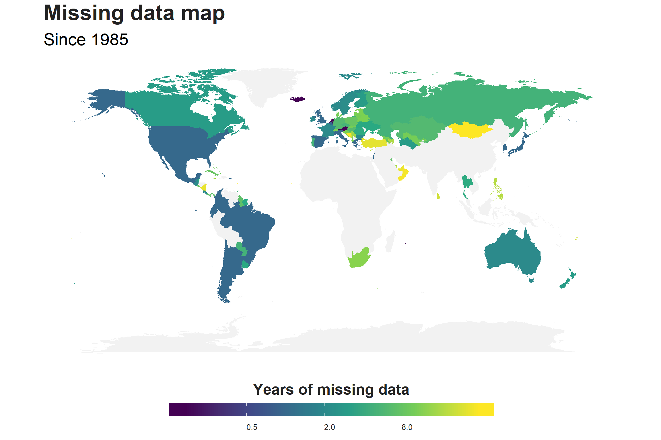
Most of the data are from Russia, America nand Europe. There are some countries that have a lot of missing data
Missing pattern
data %>%
  group_by(country, year) %>%
  summarise(na = sum(is.na(suicides_no))) %>%
  filter(na > 0) %>%
  ggplot(aes(year, country, group = country)) +
  geom_tile() +
  theme( panel.grid = element_blank()) +
  scale_x_continuous(expand = c(0,0)) +
  labs(title = "Pattern of missing data")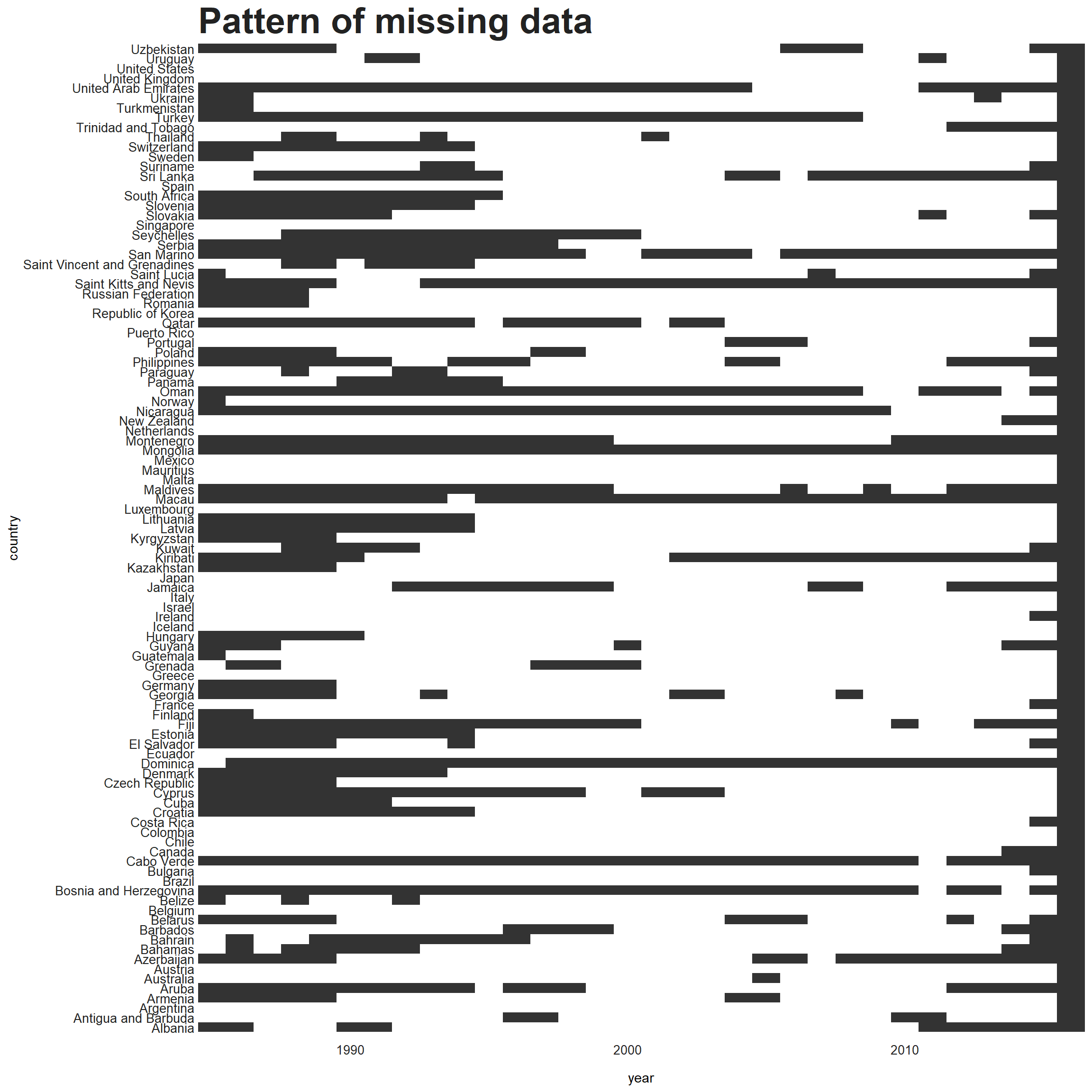
There are a lot of random missing data through out the years
What is generation’s age range?
data %>% filter(!is.na(generation)) %>%
  separate(age, into =c("min", "max")) %>% mutate(max = ifelse(max== "years", 100, max)) %>%
  mutate(min = as.integer(min), max = as.integer(max)) %>%
  mutate(min = year - min, max = year - max) %>%
  ggplot() + geom_jitter(aes(generation, min, color = "Max possible birth year"), alpha = 0.3) +
  geom_jitter(aes(generation, max, color = "Min possible birth year"), alpha = 0.3) +
  scale_color_manual(name = "", values = c("green", "red")) + theme(legend.position = "top") +
  labs(title = "Birth year of all generations", y = "Birth year", x = "Generations")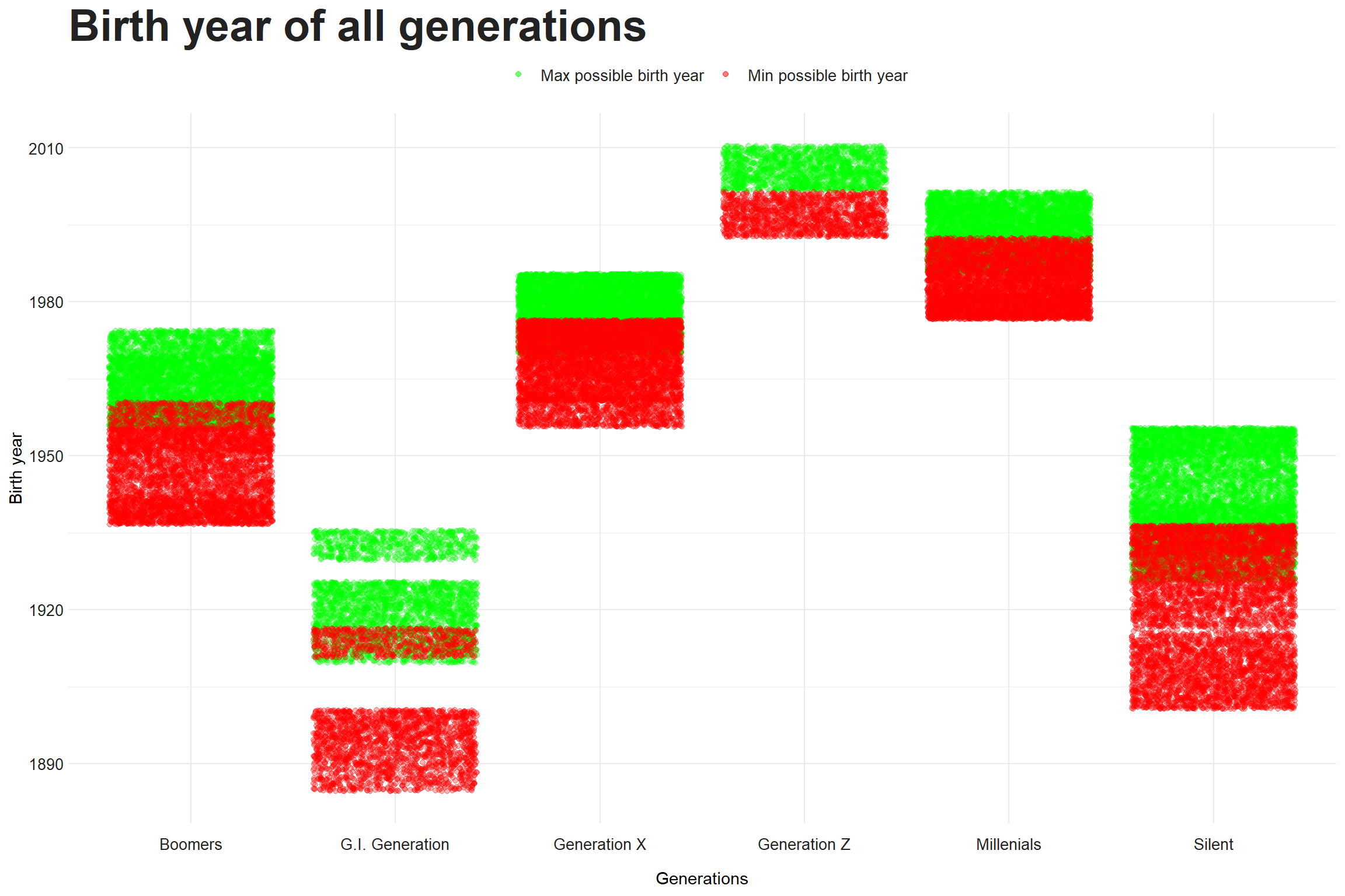
- Since Age values are not provided but put in the age range, we can only estimate the actual year birth.
From the data, birth year of :
G.I generation is aroung 1900
Silent generation is around 1925
Boomers generation is around 1955
Generation X is around 1975
Millennials is around 1980
Generation Z is around 2000
Compare to Wiki
G.I generation birth year is from 1900s to late 1920s
Silent generation birth year is from late 1920s to mid 1940s
Boomers generation birth year is from 1946 to 1964
Genration X birth year is from early-to-mid 1960s to the early 1980s
Millennials birth year is from early 1980s to early 2000s
Generation Z birth year is from 1990s till now
There is no big discrepancy between data set and Wiki, no outliner either, so it is safe to assume that there is no mistake in our data.
Analyze
Suicides rate by year all over the world
Set up data
rate <- data %>%
  group_by(country, year) %>%
  summarise(suicides_rate = sum(suicides_no)/sum(population) * 1e5) %>%
  ungroup()
Suicides rate per country per year of all recorded country visualized in boxplot.
The number on top shows number of countries recorded in each year.
rate %>%
  filter(!is.na(suicides_rate)) %>% group_by(year) %>% mutate(n = n()) %>%
  ggplot(aes(x = factor(year))) +
  geom_boxplot(aes(y = suicides_rate )) +
  geom_text(aes(label = n, y = 55)) +
  theme(axis.text.x = element_text(angle = 45)) +
  labs(title = "Distribution of suicide rate of all country", subtitle = "Since 1985" , y = "Suicide rate", x = "Year")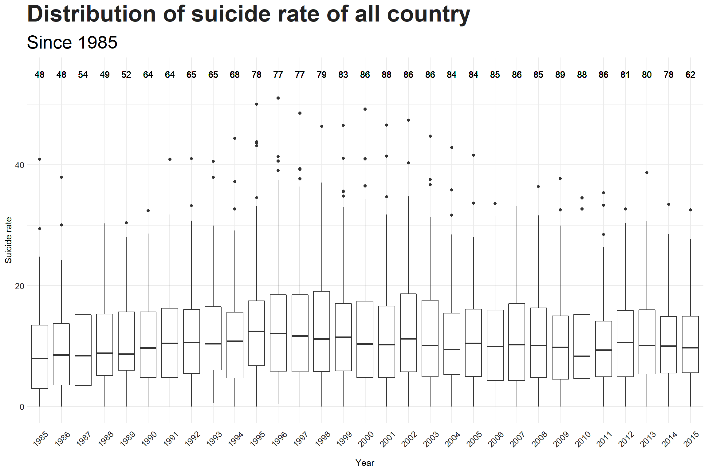
There is no noticable trend
Rate of suicides per country
rate %>%
  ggplot(aes(year, suicides_rate, color = country)) +
  geom_line() +
  geom_text_repel(data = . %>% ungroup() %>%
                    group_by(year) %>%
                    top_n(n = 5, wt = suicides_rate) %>%
                    ungroup() %>%
                    complete(country, year),
                  aes(label = country), hjust = 0,
                  segment.alpha = 0.2, xlim = c(2015,NA)) +
  coord_cartesian(clip = "off") +
  theme(legend.position = "none",
        plot.margin = margin(1,4,1,1, "cm")) +
  labs(title = "Rate of suicides", subtitle = "in {round(frame_along)}", x = "Year", y = "Suicide rate") +
transition_reveal(year) 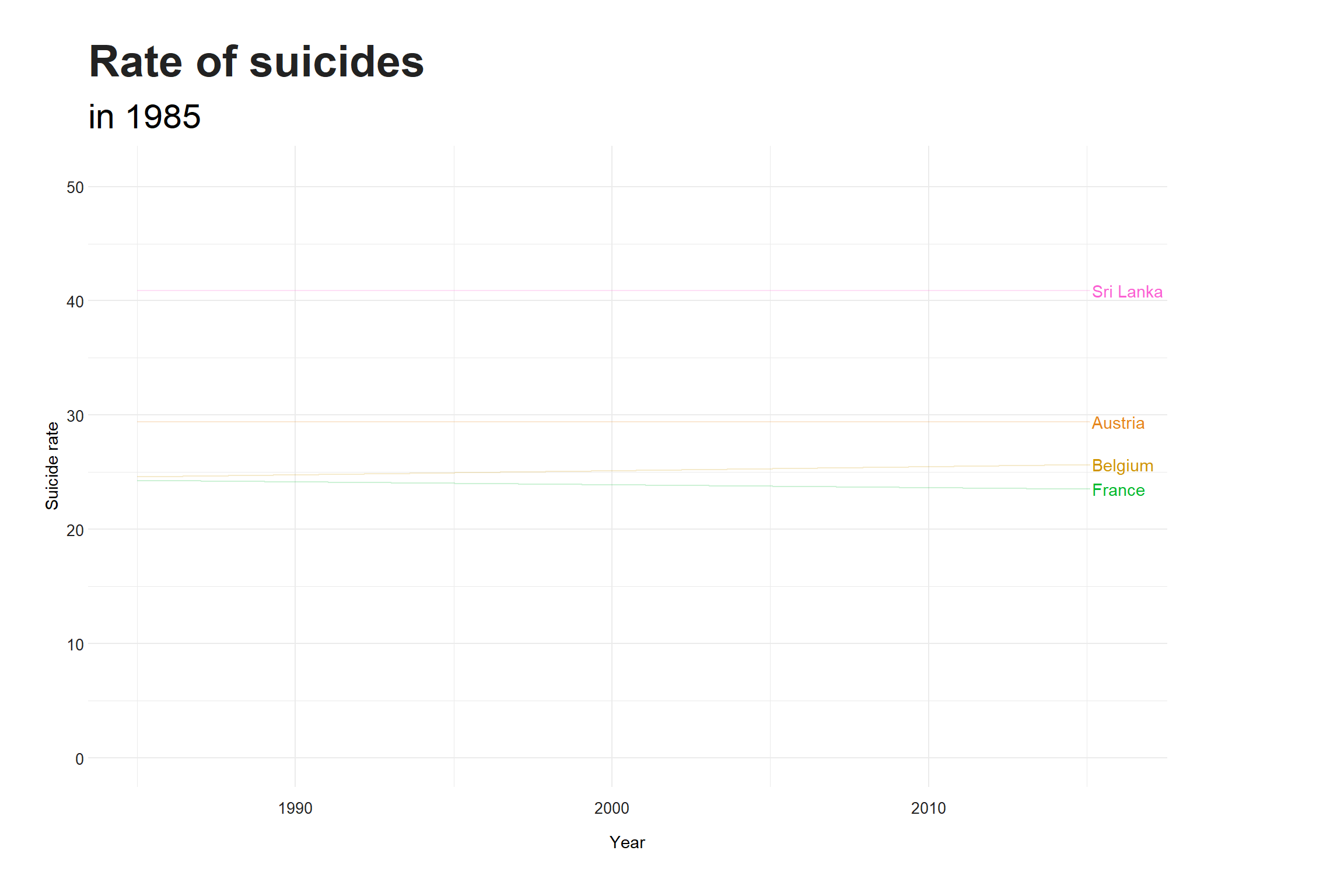
Top recorded suicide rate in each year with barplot
(rate %>% ungroup() %>%
  group_by(year) %>%
  top_n(n = 5, wt = suicides_rate) %>%
  mutate(rank = rank(-suicides_rate)) %>%
  ggplot(aes(rank, suicides_rate, fill = country)) +
  geom_col() +
  geom_label(aes(label = country ),fill = "white") +
  theme(legend.position = "none",
        panel.grid = element_blank(),
        axis.title.y = element_blank(),
        axis.text.x = element_text(size = 15),
        axis.text.y = element_text(size = 20),
        axis.title.x = element_text(size = 20)) +
  scale_x_reverse() +
  coord_flip() +
  transition_states(year, transition_length = 2, state_length = 2) +
  labs(subtitle = "in {closest_state}", title = "Top recorded suicide rate", y = "Suicide rate")+
  enter_drift(x_mod = -1) + exit_drift(x_mod = 1)) %>%
  animate(nframes = 300, height = 800, width = 800 )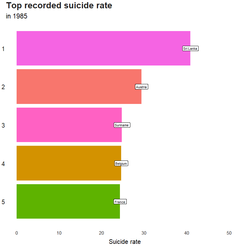
Recorded suicides rate in each year with map
(worldmap +
   geom_polygon(data = rate %>%
                  left_join(world, by = c("country" = "region")) %>%
                  filter(!is.na(suicides_rate)),
                aes(fill = suicides_rate))  +
   scale_fill_viridis_c(name = "Suicides rate",
                       guide = guide_colorbar(title.position = "top",
                                              direction = "horizontal"),
                       na.value  = "#f2f2f2") +
  theme(legend.position = "bottom",
        legend.key.width = unit(5,"cm"),
        legend.title = element_text(size = 20, face = "bold", color = "#222222"),
        legend.title.align = 0.5,
        panel.grid = element_blank(),
        plot.margin = margin(15,1,1,1),
        axis.text.x = element_blank(),
        axis.text.y = element_blank()) +
  labs(subtitle = "in {closest_state}", title = "Suicide rate worldwide")+
  transition_states(year)) %>%
  animate(duration = 20, height = 800, width = 1200)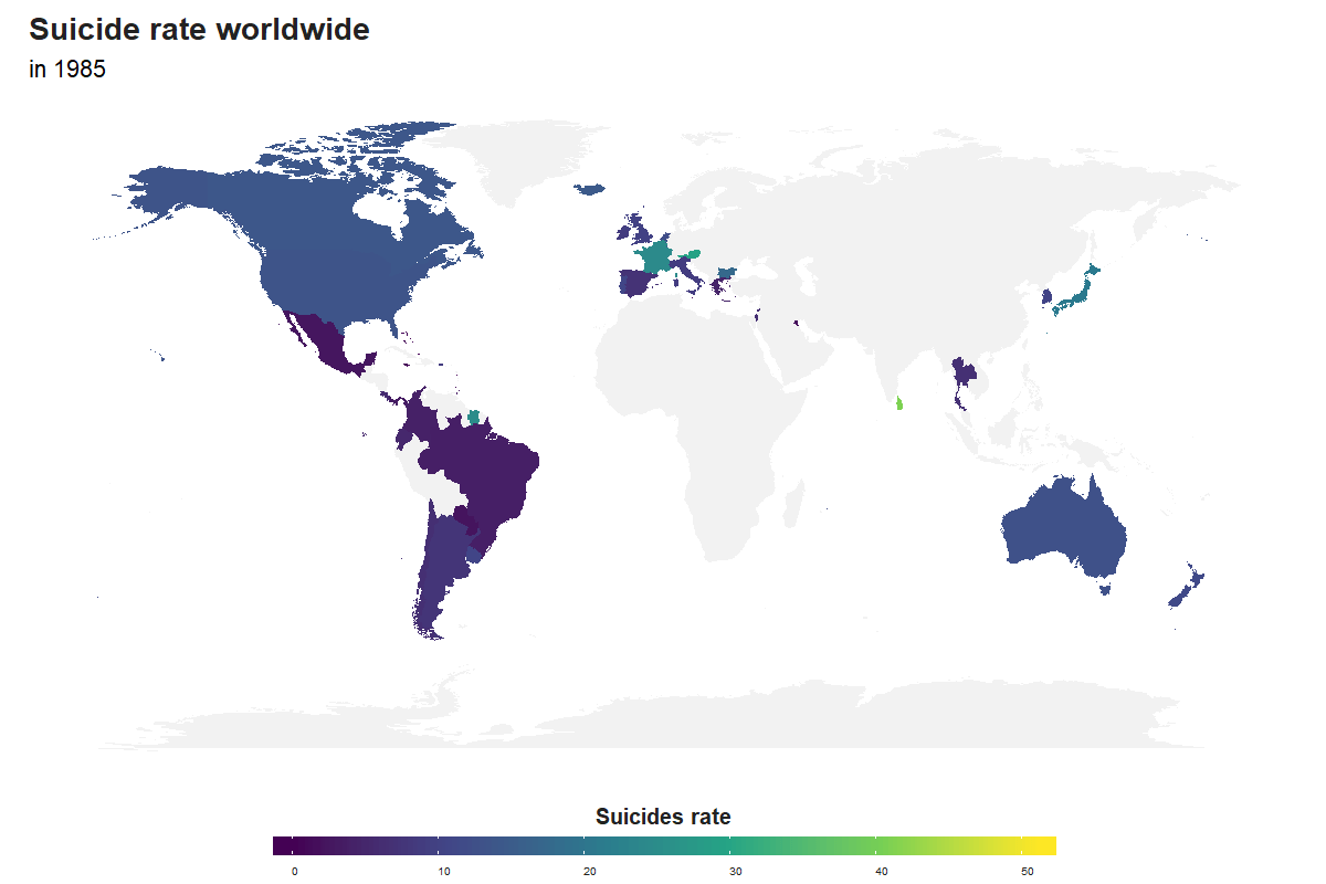
Top 10 biggest increase in suicide rate in 1 year all time
rate %>%
  mutate(lag = suicides_rate - lag(suicides_rate)) %>%
  top_n(10, lag) %>%
  arrange(desc(lag))
## # A tibble: 10 x 4
## country year suicides_rate lag
## <chr> <dbl> <dbl> <dbl>
## 1 Montenegro 2007 20.6 20.6
## 2 Montenegro 2005 20.2 20.2
## 3 Guyana 1999 24.8 19.5
## 4 Kiribati 1993 18.8 12.4
## 5 Mauritius 1987 15.4 12.2
## 6 Slovakia 2008 11.5 11.5
## 7 Suriname 2006 24.7 8.62
## 8 Suriname 1991 15.7 8.24
## 9 Saint Lucia 2009 8.13 8.13
## 10 Iceland 1990 17.1 7.66Top 10 biggest decrease in suicide rate in 1 year
rate %>%
  mutate(lag = suicides_rate - lag(suicides_rate)) %>%
  top_n(10, -lag) %>%
  arrange(lag)
## # A tibble: 10 x 4
## country year suicides_rate lag
## <chr> <dbl> <dbl> <dbl>
## 1 Montenegro 2006 0 -20.2
## 2 Slovakia 2006 0 -13.2
## 3 Kiribati 1995 3.03 -12.4
## 4 Seychelles 1986 1.74 -12.2
## 5 Suriname 1986 12.9 -11.9
## 6 Saint Vincent and Grenadines 2013 0 -9.98
## 7 Kiribati 1992 6.36 -9.80
## 8 Luxembourg 2003 11.3 -9.00
## 9 Suriname 1996 5.31 -8.82
## 10 Mauritius 1986 3.12 -8.66Based on this, more information can be obtained to get a further insight of the events in these countries
Biggest changes
(ggplot(data = rate %>% filter(country %in% (rate %>% group_by(country) %>%
  filter(!is.na(suicides_rate)) %>%
  summarise(delta = max(suicides_rate, na.rm = T) - min(suicides_rate, na.rm = T)) %>%
  arrange(desc(delta)) %>%
  top_n(10, delta) %>% pull(country))),aes(year, suicides_rate, color = country) ) +
  geom_line() +
  geom_text_repel(aes(label = country), xlim = c(2020, NA), hjust = 0, segment.alpha = 0.2) +
  coord_cartesian(clip = "off") +
  theme(legend.position = "none",
        plot.margin = margin(1, 3.5, 1, 1, "cm")) +
  labs(title = "Top changes in rate of suicide", subtitle = "in {round(frame_along)}", x = "Year", y = "Suicide rate") +
  transition_reveal(year)) %>%
  animate(duration = 20)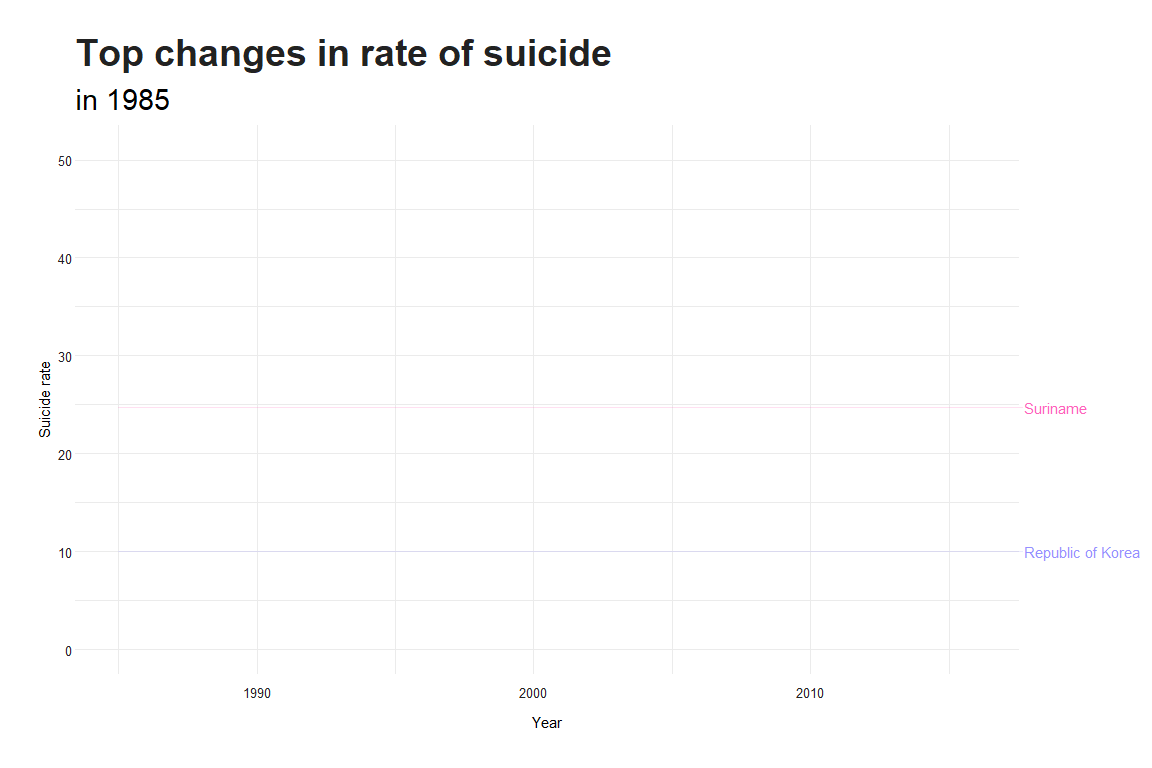
Suicide rate by GDP
rate %>% left_join(countrystat) %>%
  ggplot(aes(suicides_rate, gdp_capita)) +
  geom_point() +
  labs(y = "GDP per capita", x = "Suicide rate", title = "Suicide rate by GDP", subtitle = "Since 1985")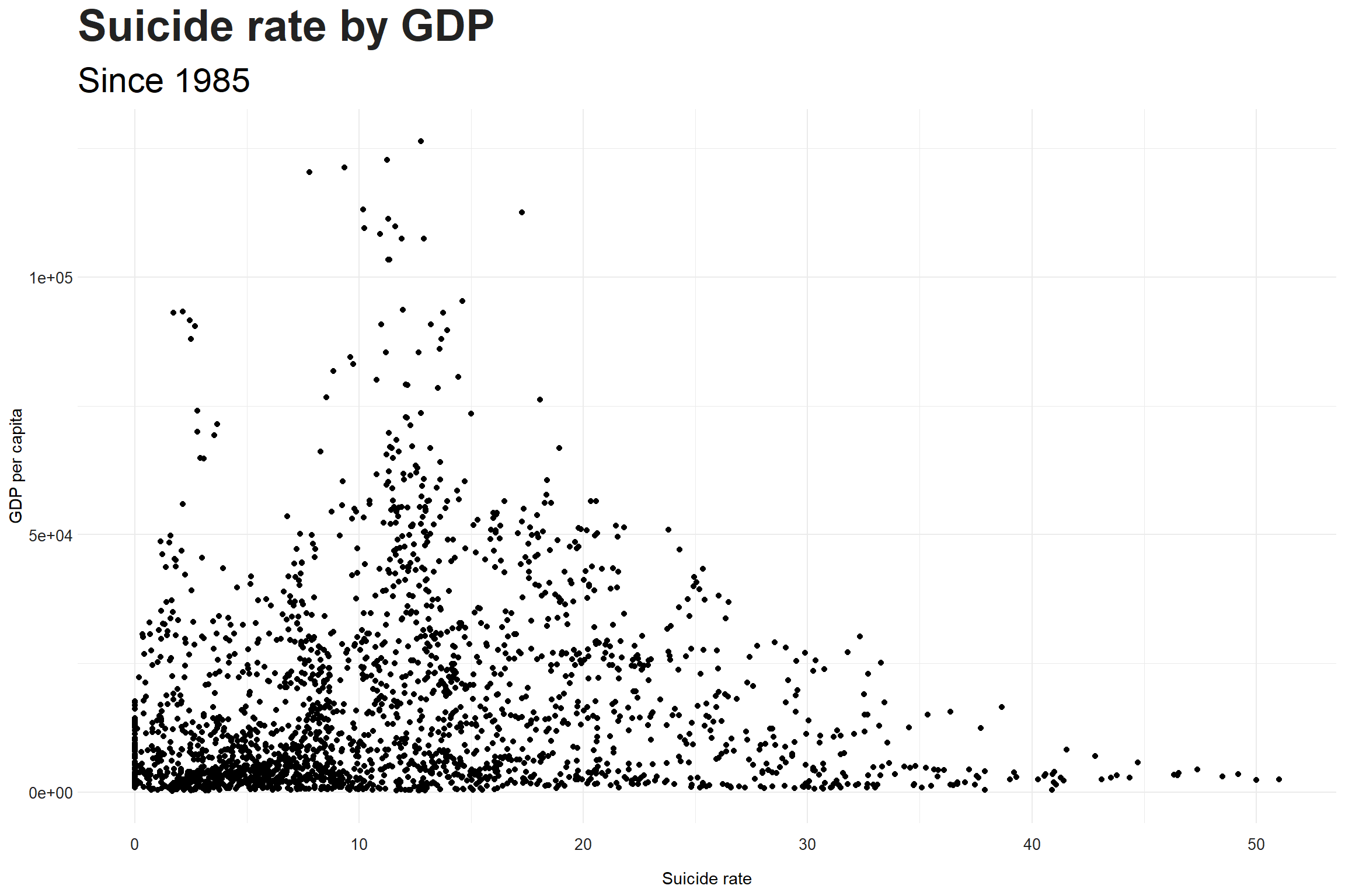
There is no indication of a relationship between them
Number of suicides per country
Prepare data
n_suicides <- data %>%
  group_by(country,year) %>%
  summarise(n = sum(suicides_no))
Number of suicides per country each year
n_suicides %>%
  ggplot(aes(year, n, color = country)) +
  geom_line() +
  geom_text_repel(data = . %>% ungroup() %>%
                    group_by(year) %>%
                    top_n(n = 5, wt = n) %>%
                    ungroup() %>%
                    complete(country, year),
                  aes(label = country ), xlim = c(2015,NA), hjust = 0,
                  segment.alpha = 0.2) +
  coord_cartesian(clip = 'off') +
  theme(legend.position = "none",
        plot.margin = margin(1,4,1,1, "cm")) +
  labs(title = "Number of suicides", subtitle = "in {round(frame_along)}", x = "Year", y = "Number of rate") +
  transition_reveal(year)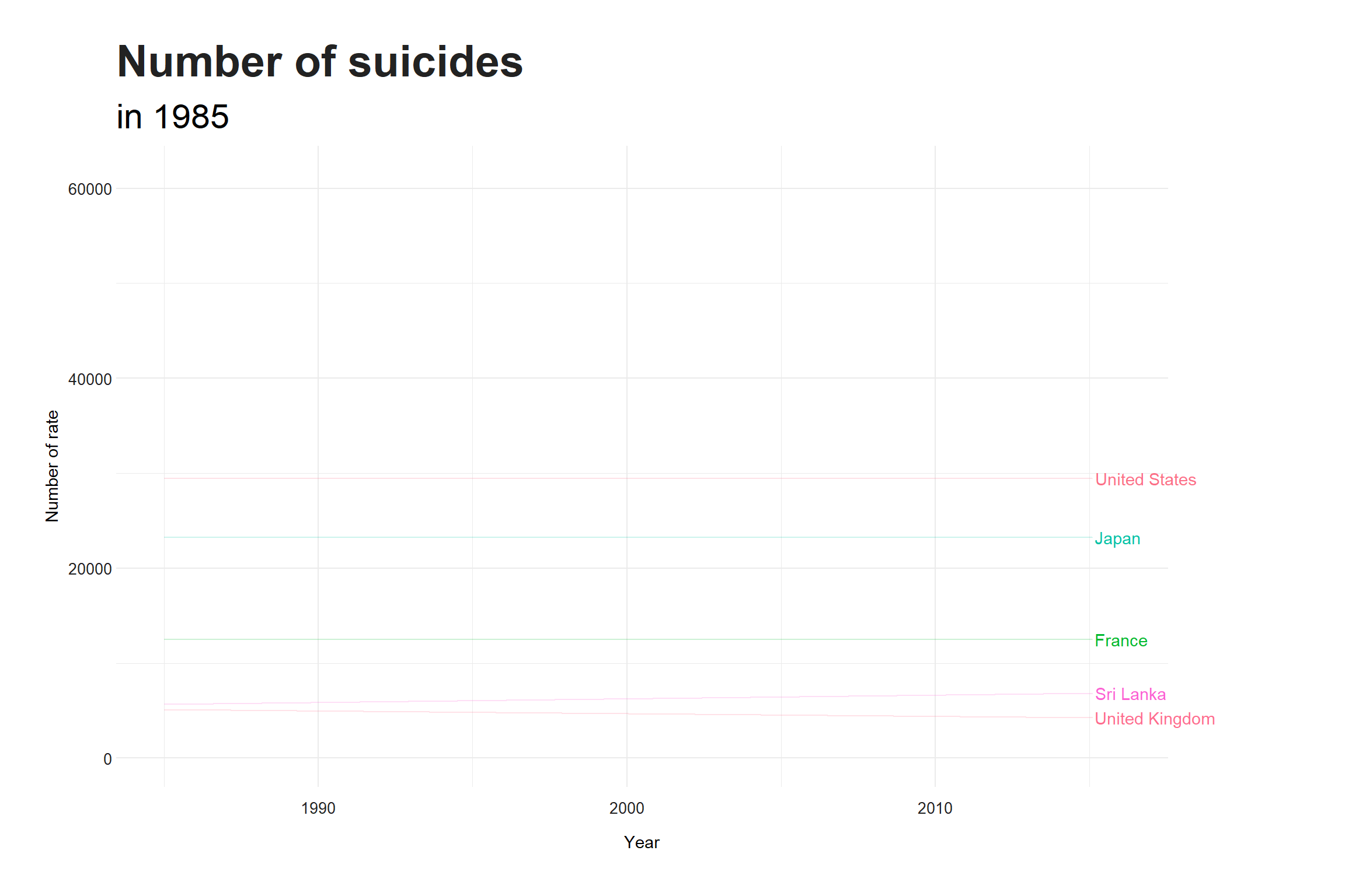
From 2010
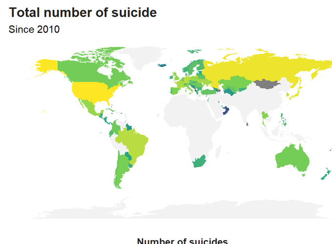
Total number of suicide since 2010
worldmap + data %>% filter(year >= 2010 & year < 2016) %>%
  group_by(country) %>%
  summarise(n = sum(suicides_no, na.rm = T)) %>%
  filter(!is.na(n)) %>%
  left_join(world, by = c("country" = "region")) %>%
  geom_polygon(data = ., aes(fill = n))  +
  scale_fill_viridis_c(name = "Number of suicides",
                       trans = "log10",
                       guide = guide_colorbar(title.position = "top",
                                              direction = "horizontal")) +
  labs(title = "Total number of suicide", subtitle = "Since 2010") +
  theme(legend.position = "bottom",
        legend.key.width = unit(5,"cm"),
        legend.title = element_text(size = 20, face = "bold", color = "#222222"),
        legend.title.align = 0.5,
        panel.grid = element_blank(),
        plot.margin = margin(15,1,1,1),
        axis.text.x = element_blank(),
        axis.text.y = element_blank())
## Warning: Transformation introduced infinite values in discrete y-axis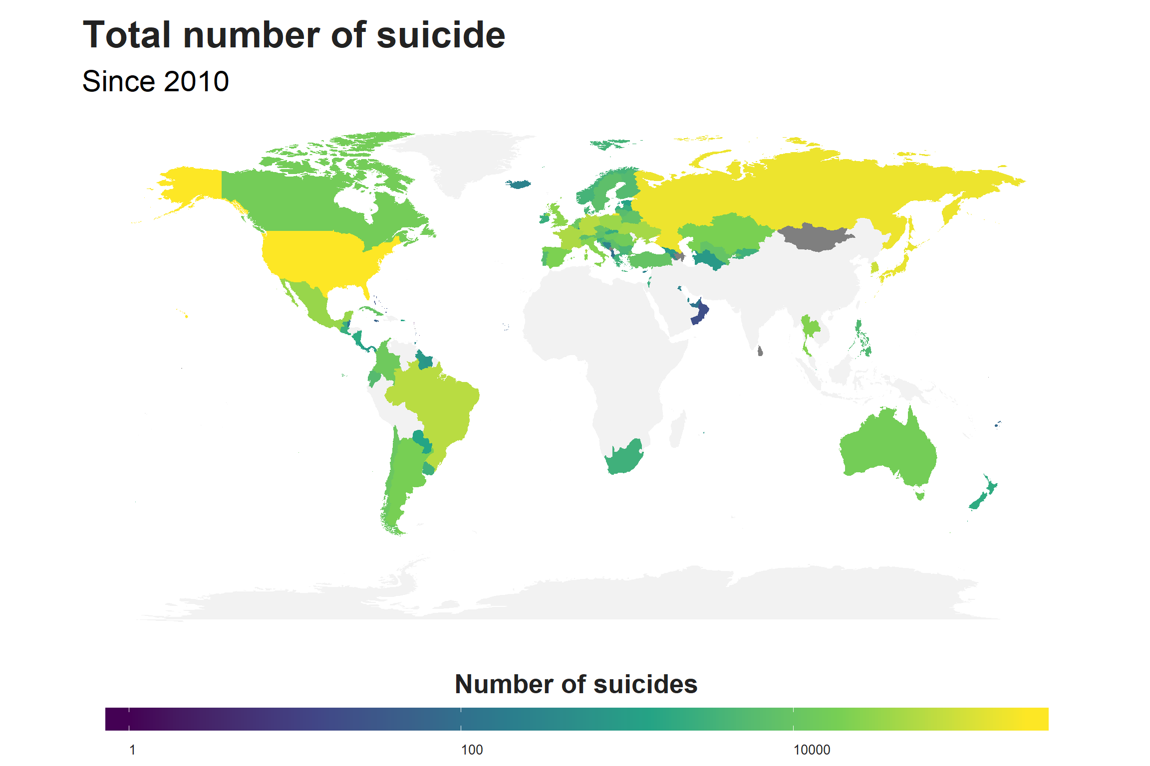
Average rate of suicide since 2010
worldmap + rate %>% filter(year >= 2010 & year < 2016) %>%
  group_by(country) %>% summarise(n = mean(suicides_rate, na.rm = T)) %>% filter(!is.na(n)) %>%
  left_join(world, by = c("country" = "region")) %>%
  geom_polygon(data = ., aes(fill = n))  +
  scale_fill_viridis_c(name = "Average rate of suicides each year",
                       guide = guide_colorbar(title.position = "top",
                                              direction = "horizontal")) +
  labs(title = "Average rate of suicide", subtitle = "Since 2010") +
  theme(legend.position = "bottom",
        legend.key.width = unit(5,"cm"),
        legend.title = element_text(size = 20, face = "bold", color = "#222222"),
        legend.title.align = 0.5,
        panel.grid = element_blank(),
        plot.margin = margin(15,1,1,1),
        axis.text.x = element_blank(),
        axis.text.y = element_blank())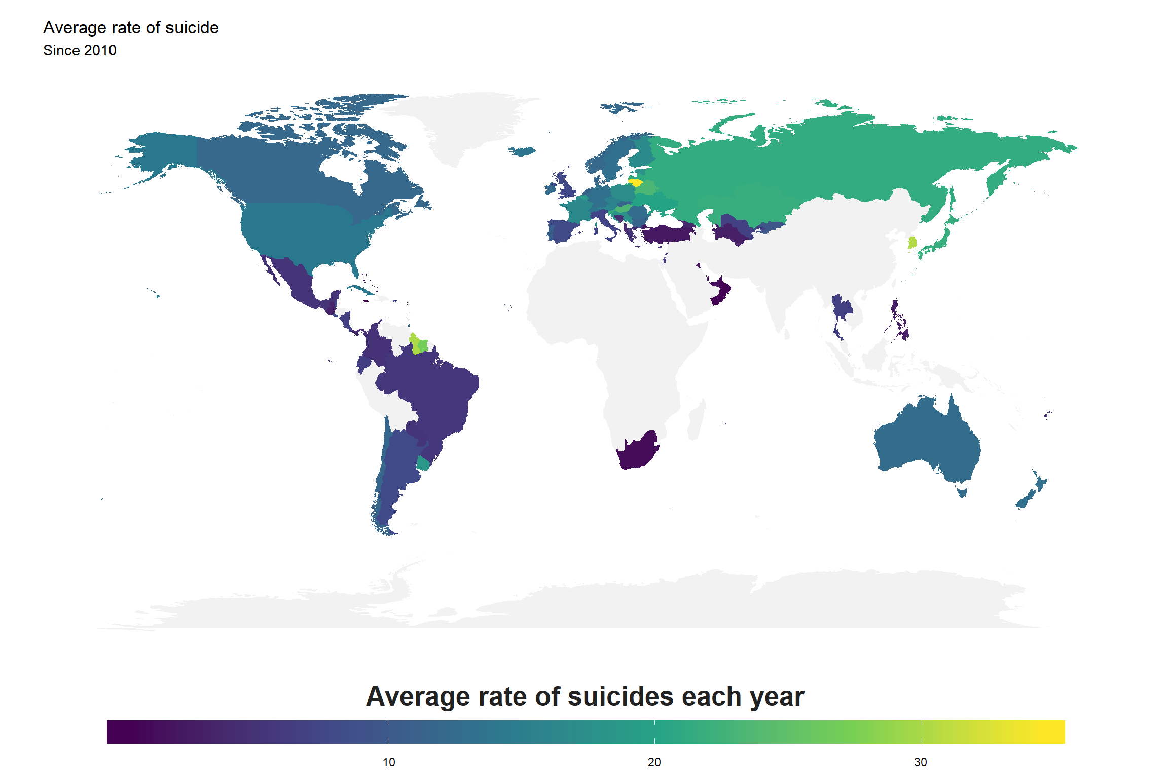
Gender
Number of suicides by gender each year in the world
data %>% group_by(year, sex) %>%
  summarise(suicides_no = sum(suicides_no, na.rm = T)) %>%
  ggplot(aes(year, suicides_no, color = sex)) +
  geom_line() +
  theme(legend.position = "none") +
  labs(title = "Number of suicide worldwide", x = "Year", y = "Suicide number", subtitle = "since 1985")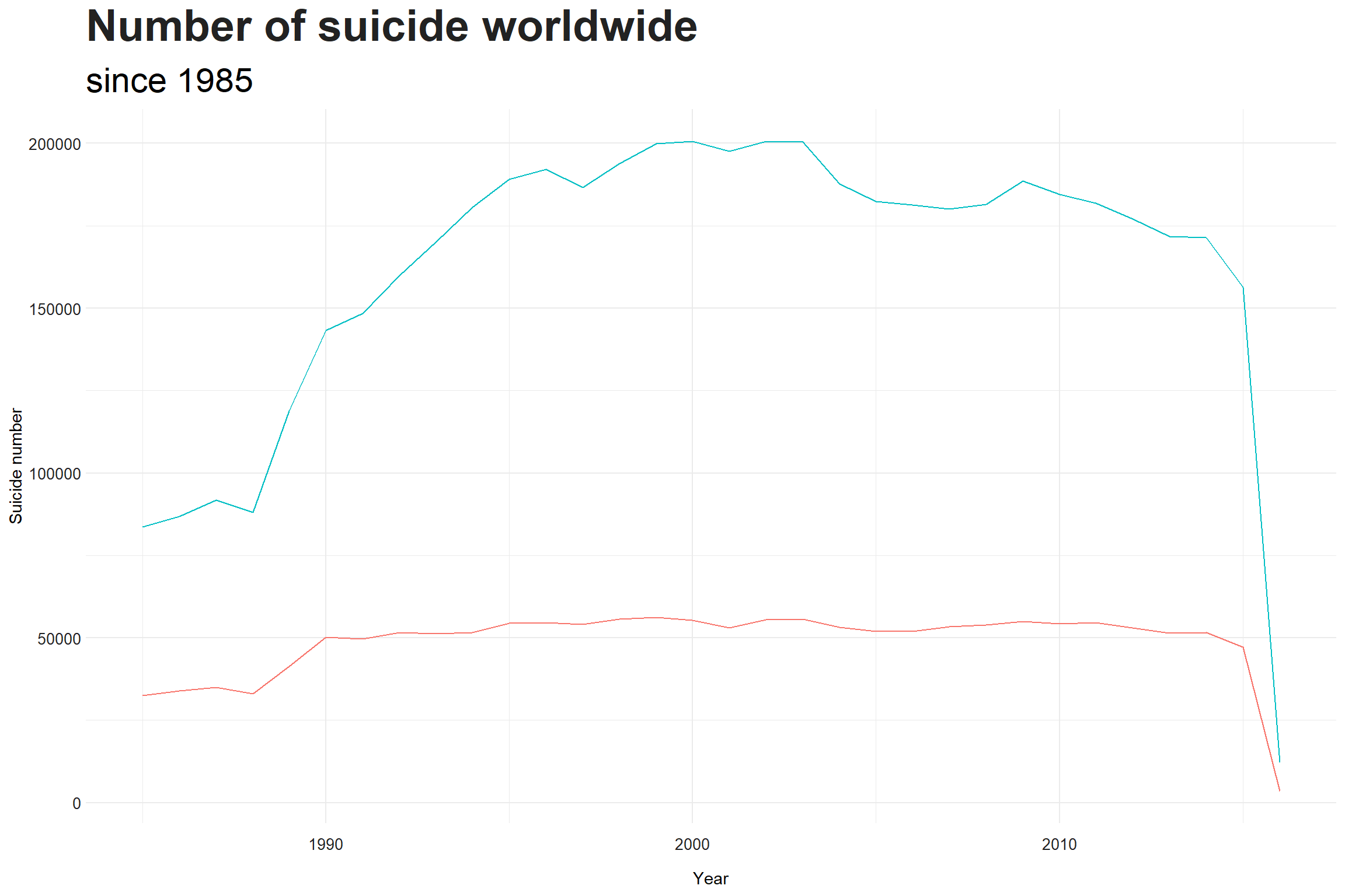
Rate of suicides by gender each year in the world
data %>% group_by(year, sex) %>%
  summarise(suicides_no = sum(suicides_no, na.rm = T)/ sum(population, na.rm = T) * 1e5) %>%
  ggplot(aes(year, suicides_no, color = sex)) +
  geom_line() +
  theme(legend.position = "none") +
  labs(title = "Rate of suicide worldwide", x = "Year", y = "Suicide rate", subtitle = "since 1985")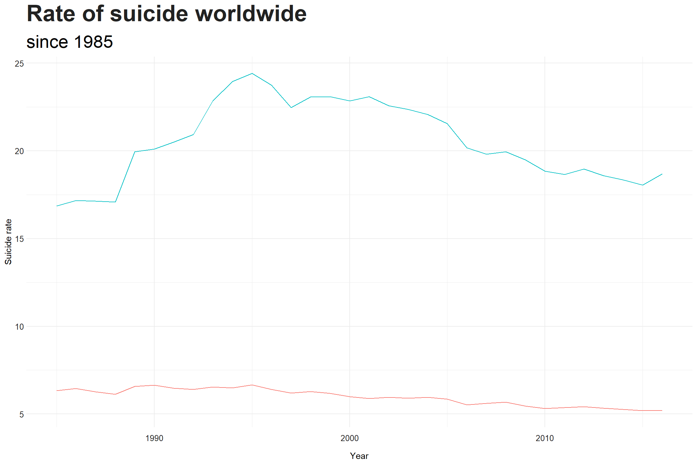
Number of suicides by gender each year in every country
data %>% group_by(country, year, sex) %>%
  summarise(suicides_no = sum(suicides_no)) %>%
  ggplot(aes(year, suicides_no, color = country)) +
  geom_line() + facet_wrap(~sex) +
  theme(legend.position = "none") +
  labs(title = "Number of suicides by gender", subtitle = "Since 1985", x = "Year",
       y = "Number of suicide")
## Warning: Removed 807 rows containing missing values (geom_path).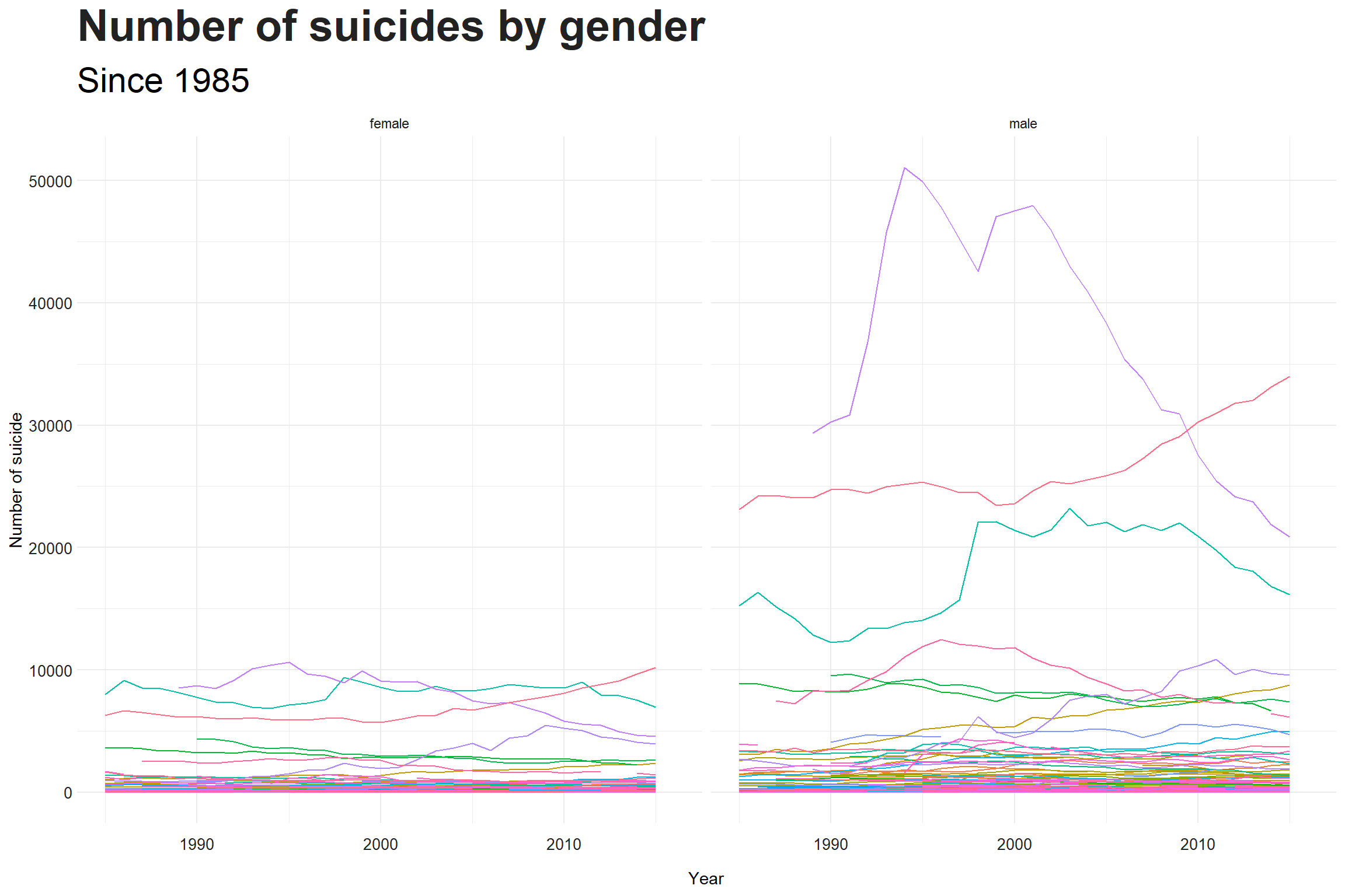
Rate of suicides by gender each year in every country
data %>% group_by(country, year, sex) %>%
  summarise(suicides_rate = sum(suicides_no)/sum(population) * 1e5) %>%
  ggplot(aes(year, suicides_rate, color = country)) +
  geom_line() + facet_wrap(~sex) +
  theme(legend.position = "none") +
  labs(title = "Rate of suicides by gender", subtitle = "Since 1985", x = "Year",
       y = "Rate of suicide")
## Warning: Removed 807 rows containing missing values (geom_path).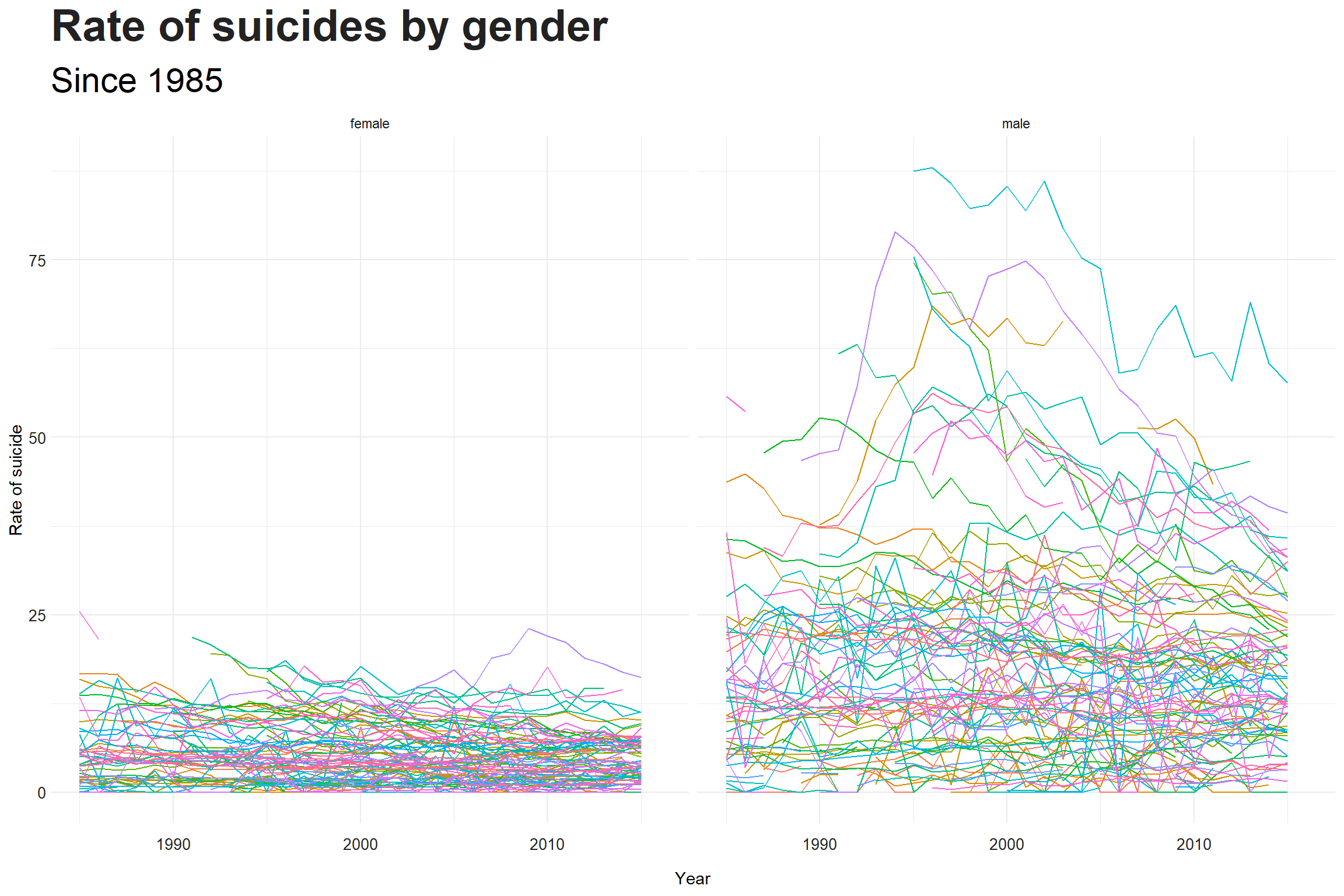
Age group
Number of suicides each age group in the world
data %>% group_by(year, age) %>%
  summarise(suicides_no = sum(suicides_no, na.rm = T)) %>%
  ggplot(aes(year, suicides_no, color = fct_reorder2(age, year, suicides_no))) +
  geom_line() +
  scale_color_discrete(name = "Age group") +
  labs(title = "Number of suicides each age group", subtitle = "Since 1985", x = "Year",
       y = "Number of suicides")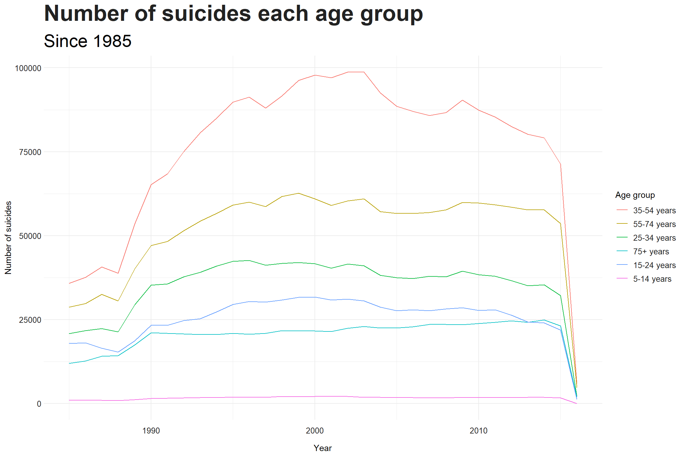
Number of suicides in 35-54 age group is the biggest due to large population proportion, in the next graph, age group 75+ actually has the highest suicide rate
Rate of suicides each age group in the world
data %>% group_by(year, age) %>%
  summarise(suicides_rate = sum(suicides_no, na.rm = T)/sum(population, na.rm = T) * 1e5) %>%
  ggplot(aes(year, suicides_rate, color = fct_reorder2(age, year, suicides_rate))) +
  geom_line() +
  scale_color_discrete(name = "Age group") +
  labs(title = "Rate of suicides each age group", subtitle = "Since 1985", x = "Year",
       y = "Rate of suicides")
## Warning: Removed 1 rows containing missing values (geom_path).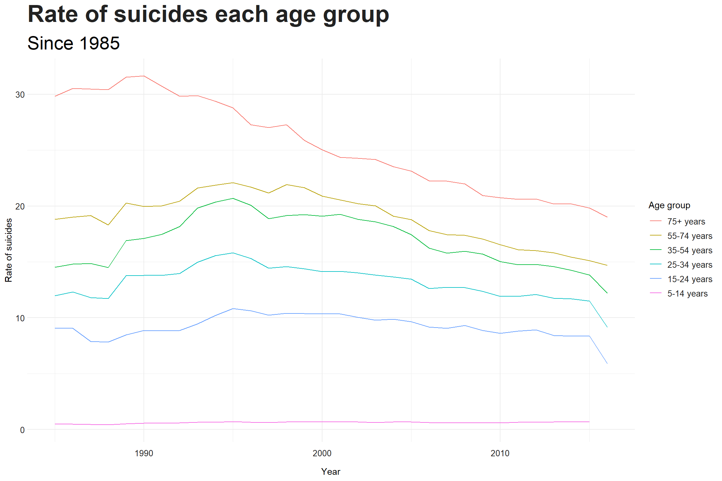
Number of suicides by age group each year in every country
data %>% group_by(country, year, age) %>%
  summarise(suicides_no = sum(suicides_no)) %>%
  ggplot(aes(year, suicides_no, color = country)) +
  geom_line() +
  geom_text_repel(data = data %>%
              group_by(country, year, age) %>%
              summarise(suicides_no = sum(suicides_no)) %>%
              filter(year == 2000) %>%
              ungroup() %>%
              group_by(age, year) %>%
              top_n(3,suicides_no),
            aes(label = country))+
  facet_wrap(~ age) +
  theme(legend.position = "none") +
  labs(title = "Number of suicides by age group", subtitle = "Since 1985",
       x = "Year", y = "Number of suicides")
## Warning: Removed 791 rows containing missing values (geom_path).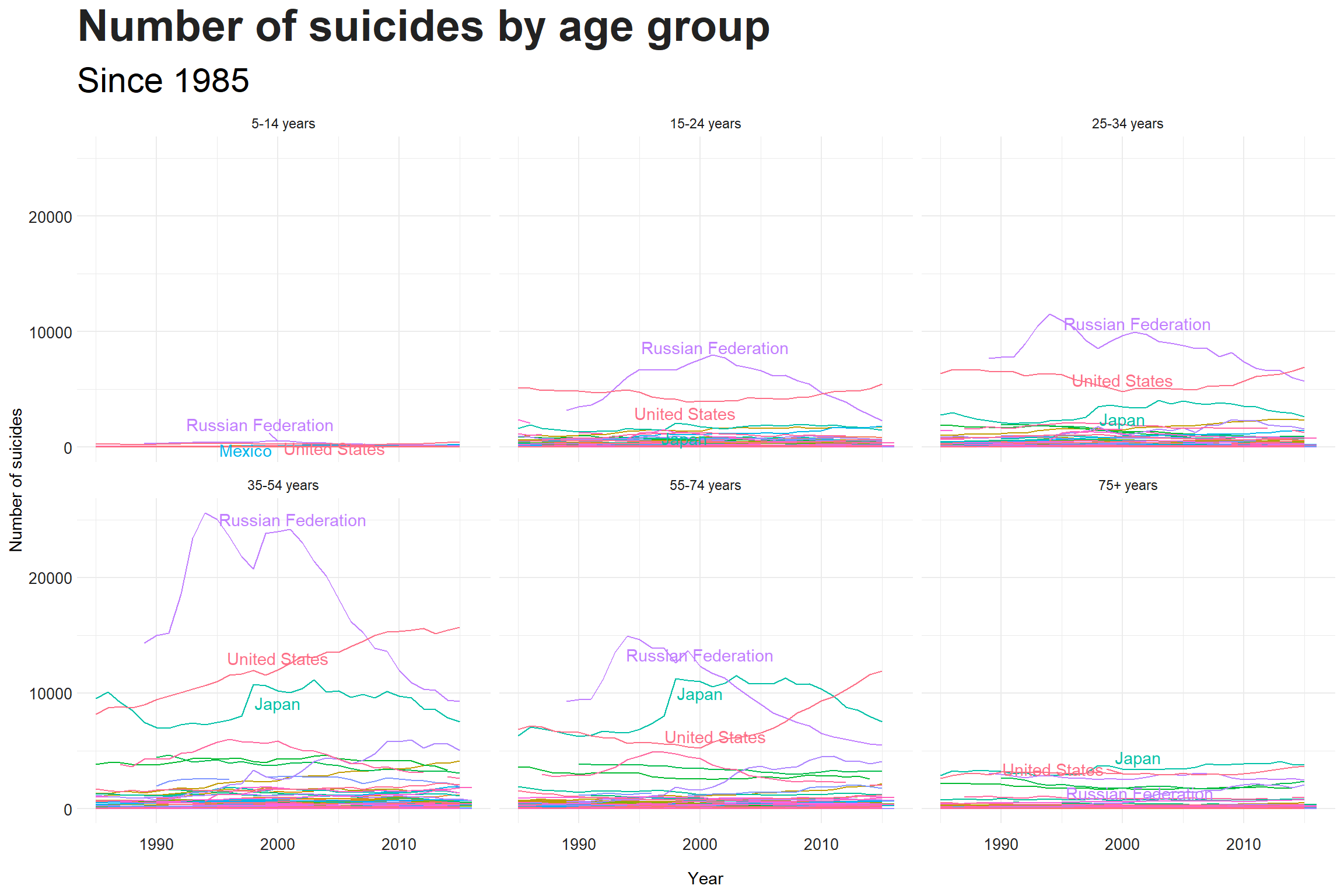
Rate of suicides by age group each year in every country
data %>% group_by(country, year, age) %>%
  summarise(suicides_rate = sum(suicides_no)/sum(population)*1e5) %>%
  ggplot(aes(year, suicides_rate, color = country)) +
  geom_line() + facet_wrap(~ age) +
  theme(legend.position = "none") +
  labs(title = "Rate of suicides by age group", subtitle = "Since 1985",
       x = "Year", y = "Rate of suicides")
## Warning: Removed 791 rows containing missing values (geom_path).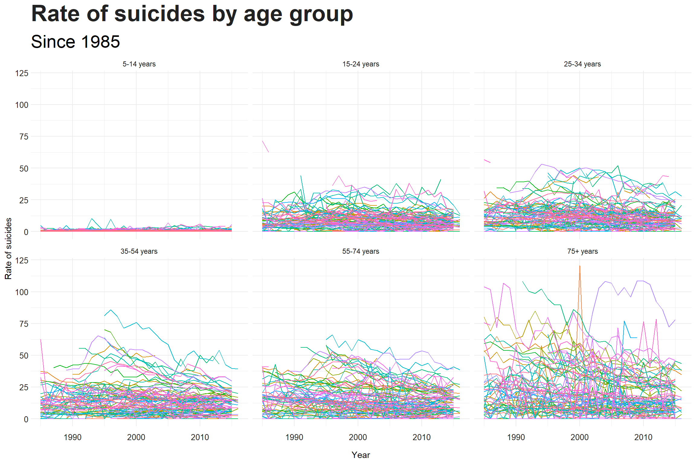
Rate of suicides by age group and sex
data %>% group_by(country, year, age, sex) %>%
  summarise(suicides_rate = sum(suicides_no)/sum(population)*1e5) %>%
  ggplot(aes(year, suicides_rate, color = country)) +
  geom_line() + facet_grid(age ~ sex)+
  theme(legend.position = "none") +
  labs(title = "Number of suicides by age and sex", subtitle = "Since 1985",
       x = "Year", y = "Number of suicides")
## Warning: Removed 823 rows containing missing values (geom_path).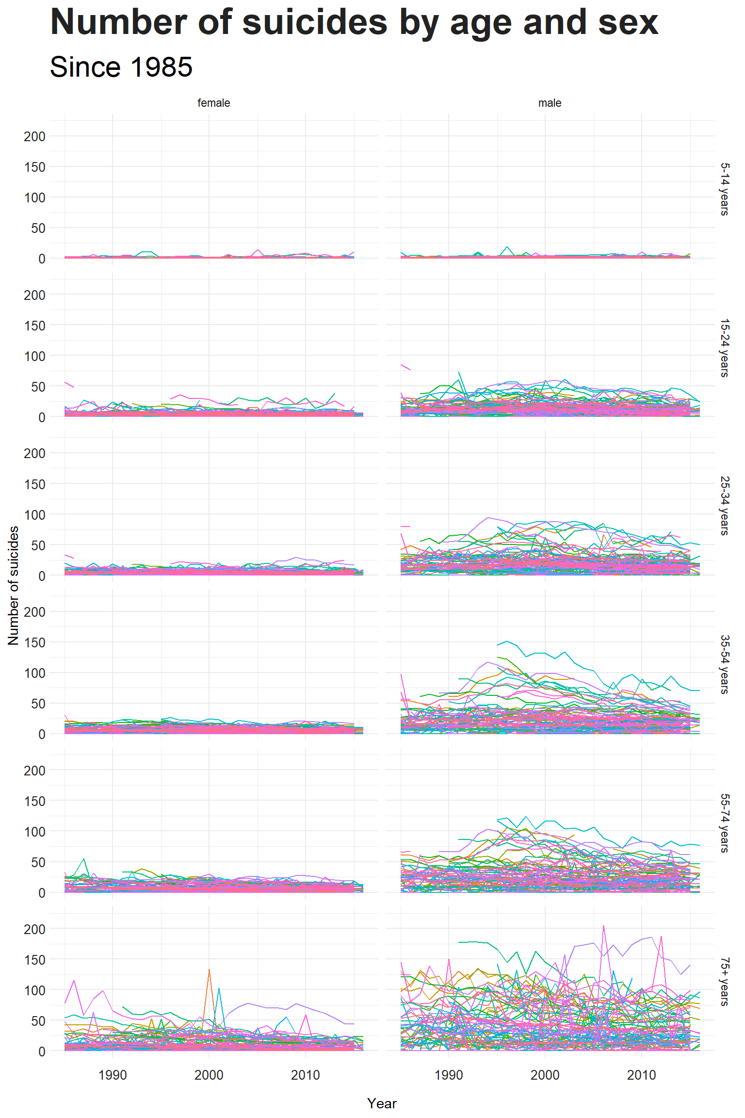
EU
EU background map
EUmap <- ggplot(data = world %>%
                  filter(region %in% eu), aes(long, lat, group = group)) + geom_polygon(fill = "#f2f2f2") +
  theme(panel.background = element_blank(),
                   axis.title = element_blank(),
                   axis.line.x = element_blank(),
                   axis.ticks = element_blank(),
                   axis.text = element_blank()) +
   coord_fixed(1.2)
Extract EU data
EUrate <- data %>%
  filter(country %in% eu) %>%
  group_by(country, year) %>%
  summarise(suicides_rate = sum(suicides_no)/sum(population) * 1e5) %>%
  ungroup()
Suicides rate per country per year of all recorded country visualized in boxplot.
The number on top shows number of countries recorded in each year.
EUrate %>%
  filter(!is.na(suicides_rate)) %>% group_by(year) %>% mutate(n = n()) %>%
  ggplot(aes(x = factor(year))) +
  geom_boxplot(aes(y = suicides_rate )) +
  geom_text(aes(label = n, y = 0.0006)) +
  geom_line(data = rate %>%
              group_by(year) %>%
              summarise(suicides_rate = median(suicides_rate, na.rm = T)),
            aes(x= factor(year), y = suicides_rate, group = "The World"), color = "red", size = 1) +
  geom_text(aes(factor(2010), 7, label = "The world median"), color = "red", size = 4) +
  theme(axis.text.x = element_text(angle = 45)) +
  labs(title = "Distribution of suicide rate of all country", subtitle = "Since 1985 in EU" , y = "Suicide rate", x = "Year")
## Warning: Removed 1 rows containing missing values (geom_path).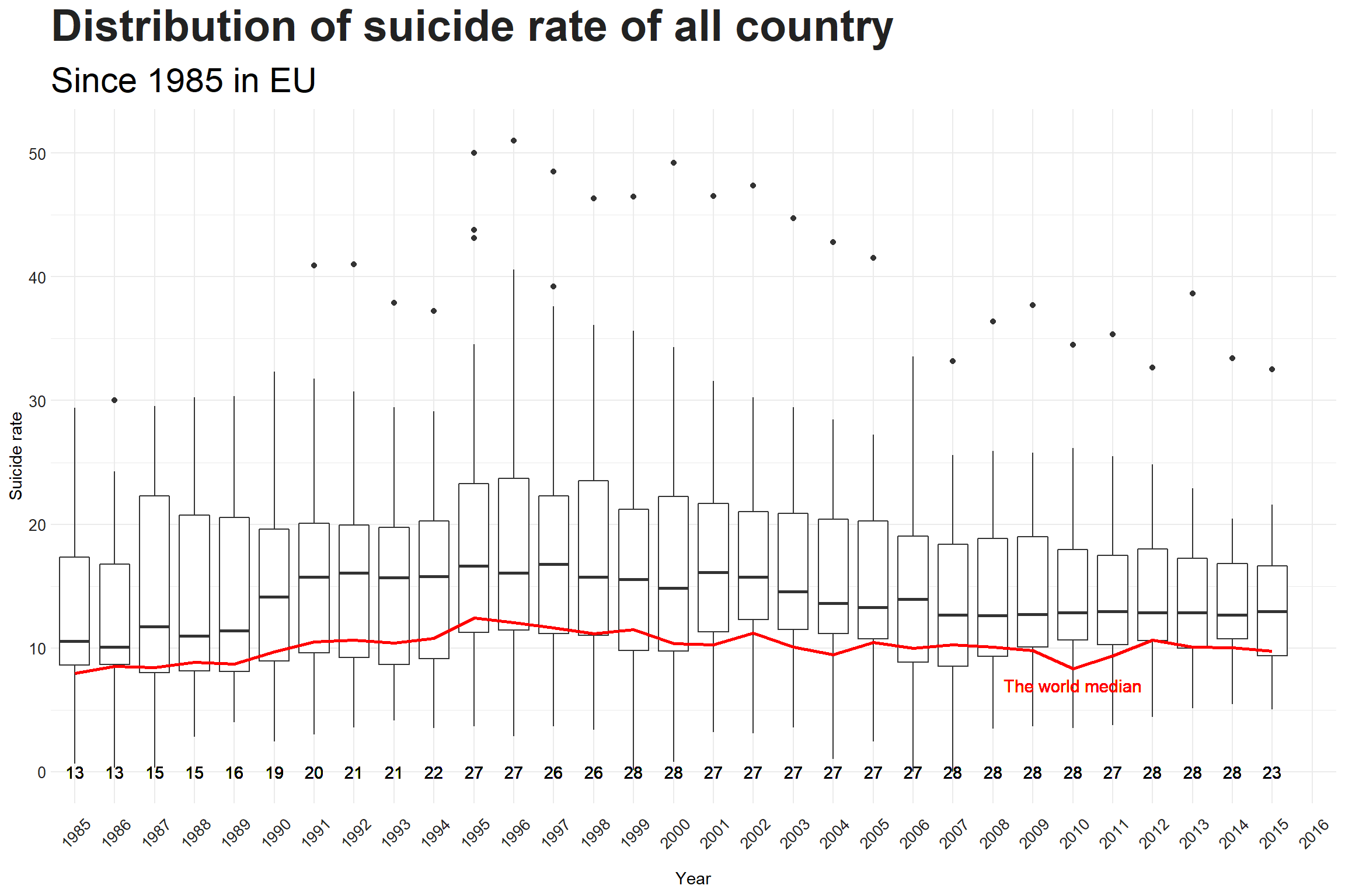
EU has higher suicides rate than the world
Rate of suicides per country
EUrate %>%
  ggplot(aes(year, suicides_rate, color = country)) +
  geom_line() +
  geom_text_repel(data = . %>% ungroup() %>%
                    group_by(year) %>%
                    top_n(n = 5, wt = suicides_rate) %>%
                    ungroup() %>%
                    complete(country, year),
                  aes(label = country), hjust = 0,
                  segment.alpha = 0.2, xlim = c(2015,NA)) +
  coord_cartesian(clip = "off") +
  theme(legend.position = "none",
        plot.margin = margin(1,4,1,1, "cm")) +
  labs(title = "Rate of suicides in EU", subtitle = "in {round(frame_along)}", x = "Year", y = "Suicide rate") +
transition_reveal(year) 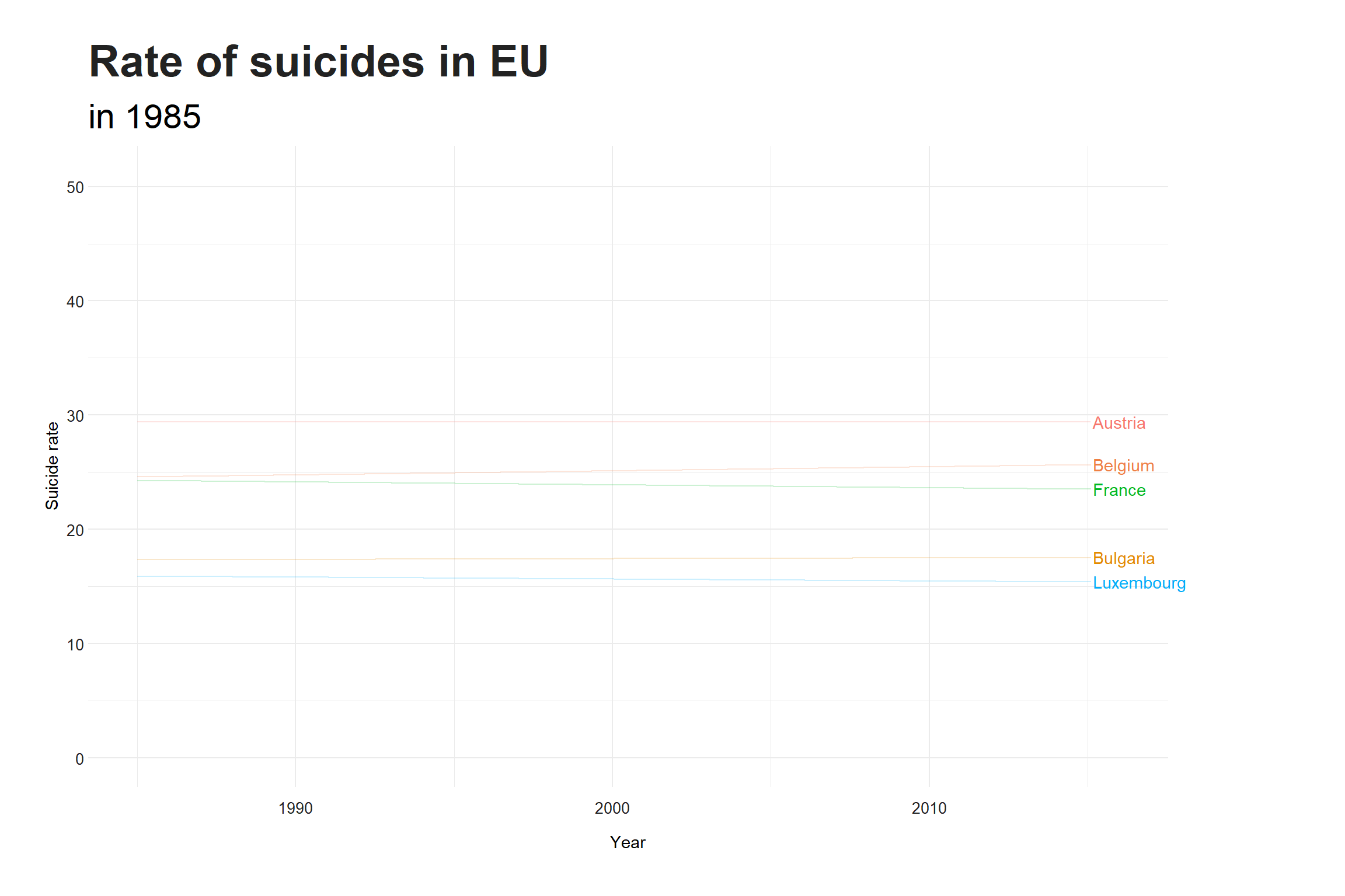
Top recorded suicides rate in each year with barplot
(EUrate %>% ungroup() %>%
  group_by(year) %>%
  top_n(n = 5, wt = suicides_rate) %>%
  mutate(rank = rank(-suicides_rate)) %>%
  ggplot(aes(rank, suicides_rate, fill = country)) +
  geom_col() +
  geom_label(aes(label = country ),fill = "white") +
  theme(legend.position = "none",
        panel.grid = element_blank(),
        axis.title.y = element_blank(),
        axis.text.x = element_text(size = 15),
        axis.text.y = element_text(size = 20),
        axis.title.x = element_text(size = 20)) +
  scale_x_reverse() +
  coord_flip() +
  transition_states(year, transition_length = 2, state_length = 2) +
  labs(subtitle = "in {closest_state}", title = "Top recorded suicide rate", y = "Suicide rate") +
  enter_drift(x_mod = 6) + exit_drift(x_mod = -1)) %>%
  animate(nframes = 300, height = 800, width = 800 )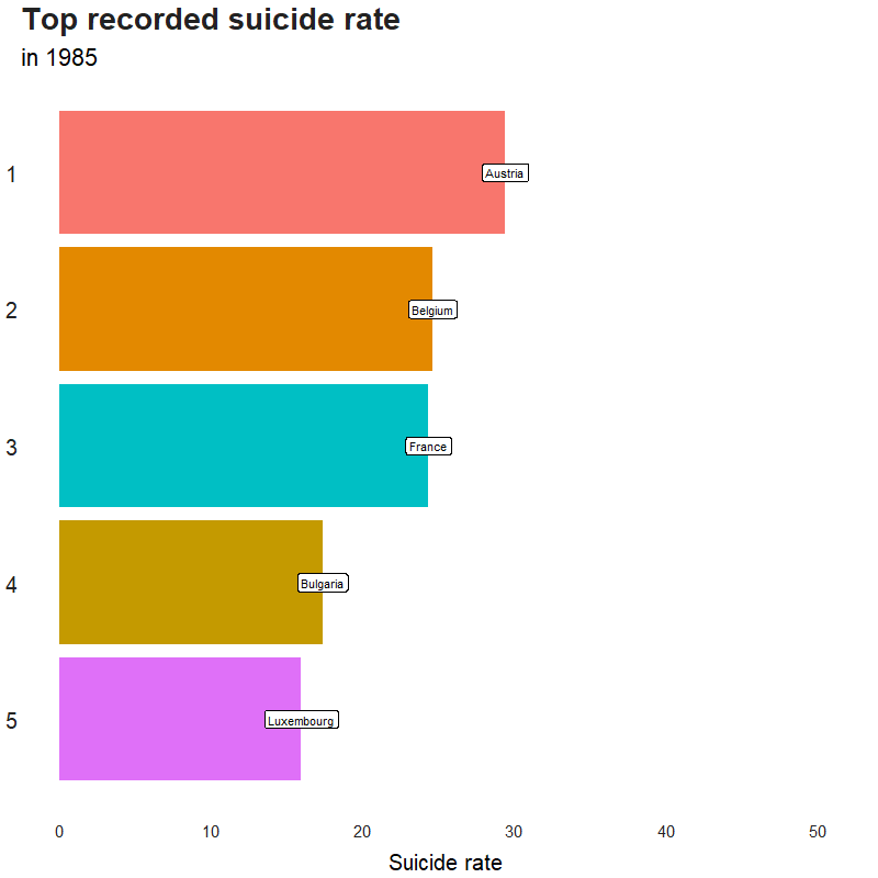
Recorded suicides rate in each year with map
(EUmap +
   geom_polygon(data = EUrate %>%
                  left_join(world, by = c("country" = "region")) %>%
                  filter(!is.na(suicides_rate)),
                aes(fill = suicides_rate))  +
   scale_fill_viridis_c(name = "Suicides rate",
                       guide = guide_colorbar(title.position = "top",
                                              direction = "horizontal"),
                       na.value  = "#f2f2f2") +
  theme(legend.position = "bottom",
        legend.key.width = unit(5,"cm"),
        legend.title = element_text(size = 20, face = "bold", color = "#222222"),
        legend.title.align = 0.5,
        panel.grid = element_blank(),
        plot.margin = margin(15,1,1,1),
        axis.text.x = element_blank(),
        axis.text.y = element_blank()) +
  labs(subtitle = "in {closest_state}", title = "Suicide rate in EU") +
  transition_states(year)) %>%
  animate(duration = 20, height = 800, width = 1200)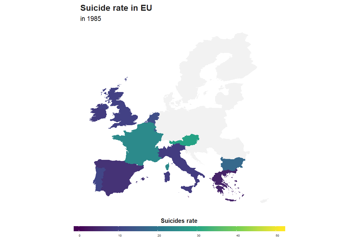
Top 10 biggest increase in suicide rate in 1 year all time
EUrate %>%
  mutate(lag = suicides_rate - lag(suicides_rate)) %>%
  top_n(10, lag) %>%
  arrange(desc(lag))
## # A tibble: 10 x 4
## country year suicides_rate lag
## <chr> <dbl> <dbl> <dbl>
## 1 Slovakia 2008 11.5 11.5
## 2 Luxembourg 1987 21.2 6.44
## 3 Lithuania 2013 38.7 5.99
## 4 Malta 2009 9.16 5.57
## 5 Luxembourg 2014 12.8 4.96
## 6 Portugal 2002 12.3 4.51
## 7 Malta 1989 7.10 4.29
## 8 Malta 1999 7.59 4.20
## 9 Latvia 2008 25.5 3.85
## 10 Luxembourg 2006 14.6 3.41Top 10 biggest decrease in suicide rate in 1 year
EUrate %>%
  mutate(lag = suicides_rate - lag(suicides_rate)) %>%
  top_n(10, -lag) %>%
  arrange(lag)
## # A tibble: 10 x 4
## country year suicides_rate lag
## <chr> <dbl> <dbl> <dbl>
## 1 Slovakia 2006 0 -13.2
## 2 Luxembourg 2003 11.3 -9.00
## 3 Lithuania 2006 33.6 -7.99
## 4 Luxembourg 2008 9.34 -7.92
## 5 Estonia 2000 28.3 -7.38
## 6 Lithuania 2014 33.4 -5.22
## 7 Luxembourg 1992 16.1 -5.15
## 8 Slovenia 2007 22.5 -5.05
## 9 Malta 1990 2.44 -4.66
## 10 Luxembourg 1998 16.1 -4.55Based on this, more information can be obtained to get a further insight of the events in these countries
Biggest changes
(ggplot(data = EUrate %>%
          filter(country %in%
                   (EUrate %>% group_by(country) %>%
                      filter(!is.na(suicides_rate)) %>%
                      summarise(delta = max(suicides_rate, na.rm = T) - min(suicides_rate, na.rm = T)) %>%
                      arrange(desc(delta)) %>%
                      top_n(5, delta) %>% pull(country))),
        aes(year, suicides_rate, color = country)) +
  geom_line() +
  geom_text_repel(aes(label = country), xlim = c(2020, NA), hjust = 0, segment.alpha = 0.2) +
  coord_cartesian(clip = "off") +
  theme(legend.position = "none",
        plot.margin = margin(1, 3.5, 1, 1, "cm")) +
  labs(title = "Top changes in rate of suicide", subtitle = "in {round(frame_along)} in EU", x = "Year",
       y = "Suicide rate") +
  transition_reveal(year)) %>%
  animate(duration = 20)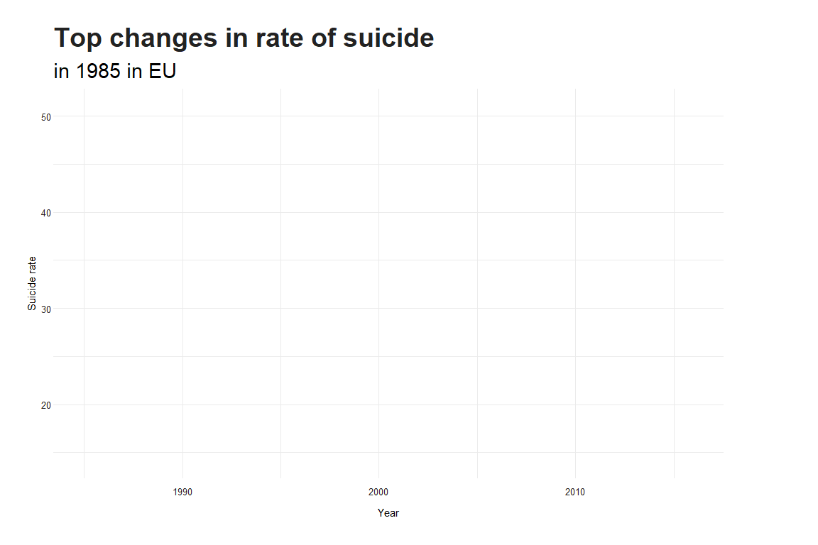
Suicide rate by GDP
EUrate %>% left_join(countrystat) %>%
  ggplot(aes(suicides_rate, gdp_capita)) +
  geom_point() +
  labs(y = "GDP per capita", x = "Suicide rate", title = "Suicide rate by GDP in EU", subtitle = "Since 1985")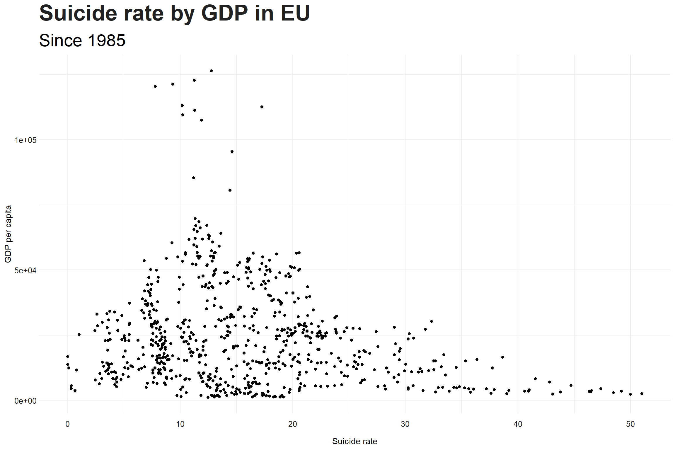
There is no indication of a relationship between them
Rate of suicides by gender each year in the EU
data %>%
  group_by(year, sex) %>%
  summarise(suicides_no = sum(suicides_no, na.rm = T)/ sum(population, na.rm = T) * 1e5) %>%
  ggplot(aes(year, suicides_no, color = sex)) +
  geom_line(aes(linetype = "Worldwide")) +
  geom_line(data = data %>%
              filter(country  %in% eu) %>%
              group_by(year, sex) %>%
              summarise(suicides_no = sum(suicides_no, na.rm = T)/ sum(population, na.rm = T) * 1e5), aes(linetype = "EU")) +
  scale_linetype_manual(name = "Region" ,values = c("Worldwide" = 2, "EU" = 1)) +
  labs(title = "Rate of suicide by gender", subtitle = "Since 1985 in EU and worldwide",
       x = "Year", y = "Rate of suicide")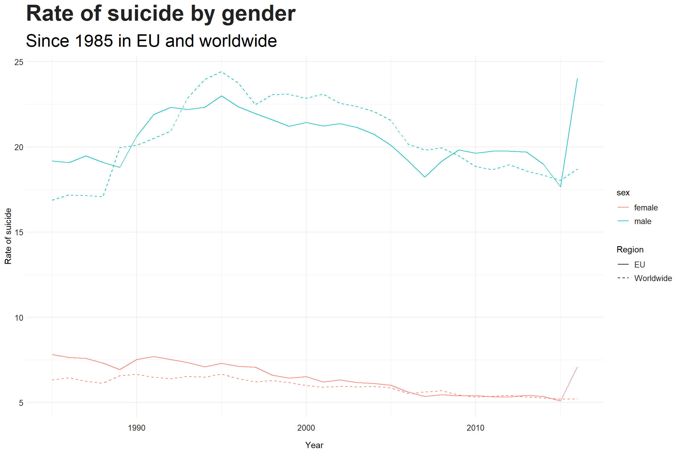
Rate of suicides by gender each year in every country
data %>%
  filter(country %in% eu) %>%
  group_by(country, year, sex) %>%
  summarise(suicides_rate = sum(suicides_no)/sum(population) * 1e5) %>%
  ggplot(aes(year, suicides_rate, color = country)) +
  geom_line() + facet_wrap(~sex) +
  theme(legend.position = "none") +
  labs(title = "Rate of suicide by gender", subtitle = "Since 1985 in EU",
       x = "Year", y = "Rate of suicide")
## Warning: Removed 142 rows containing missing values (geom_path).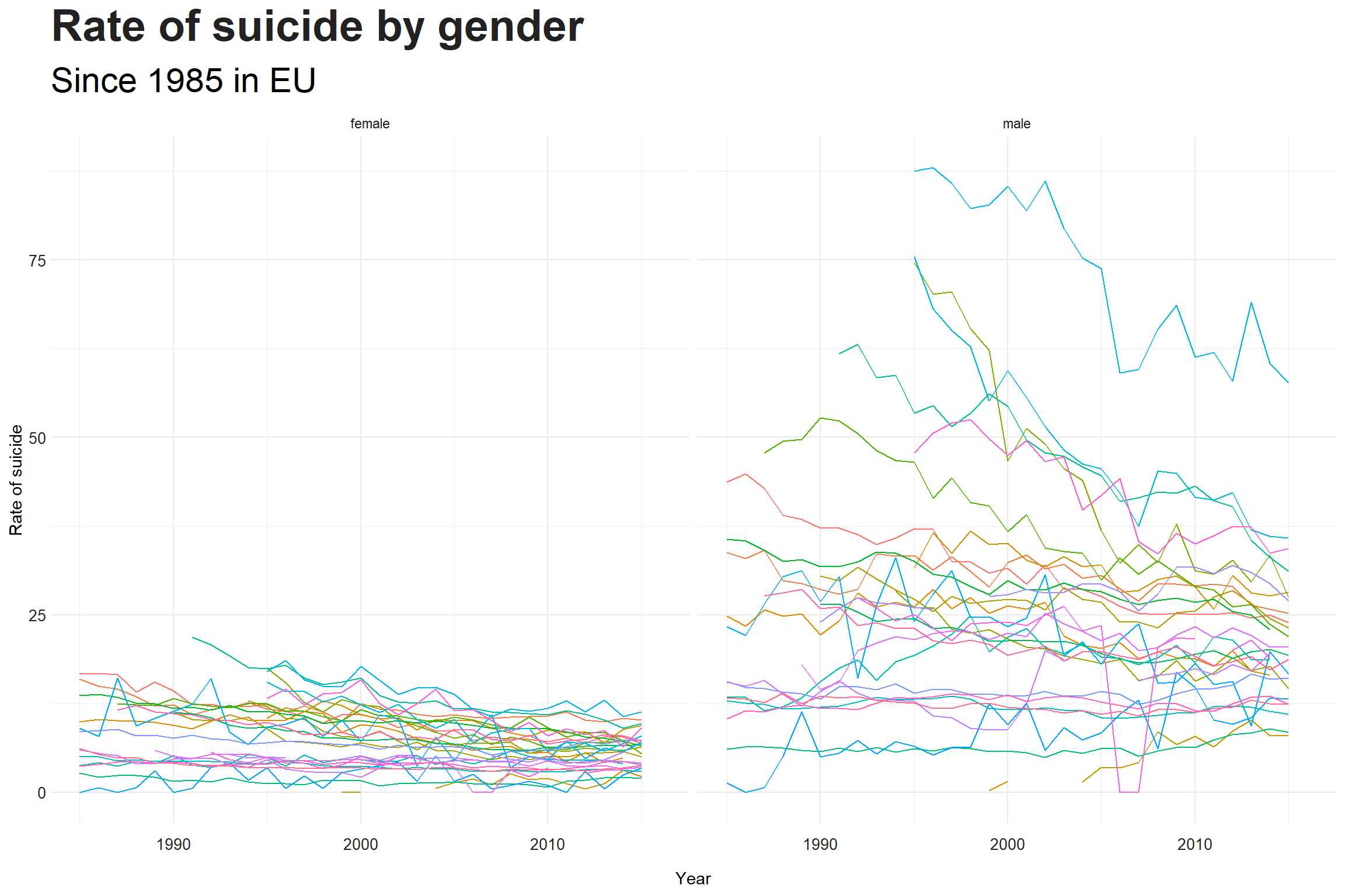
Rate of suicides by age group each year in every country
data %>%
  filter(country %in% eu) %>%
  group_by(country, year, age) %>%
  summarise(suicides_rate = sum(suicides_no)/sum(population)*1e5) %>%
  ggplot(aes(year, suicides_rate, color = country)) +
  geom_line() + facet_wrap(~ age) +
  theme(legend.position = "none") +
  labs(title = "Rate of suicide by age", subtitle = "Since 1985 in EU",
       x = "Year", y = "Rate of suicide")
## Warning: Removed 133 rows containing missing values (geom_path).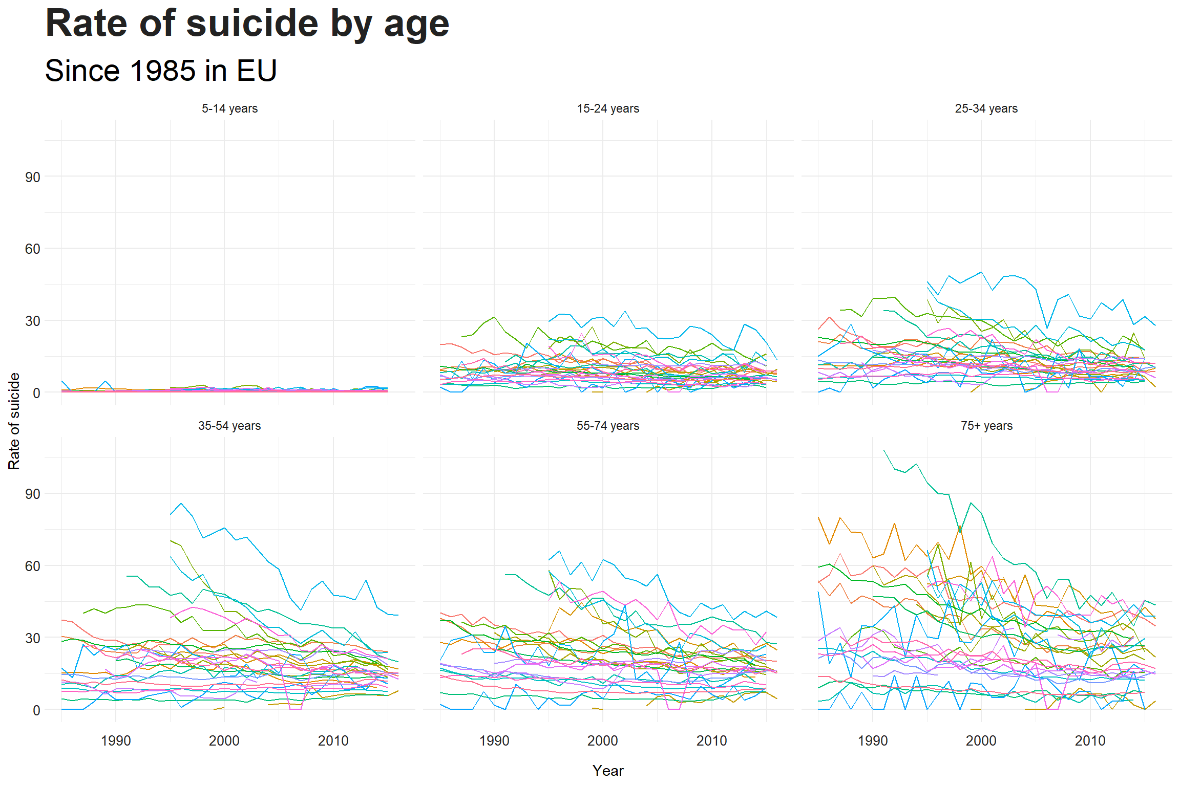
Rate of suicides by age group and sex
data %>%
  filter(country %in% eu) %>%
  group_by(country, year, age, sex) %>%
  summarise(suicides_rate = sum(suicides_no)/sum(population)*1e5) %>%
  ggplot(aes(year, suicides_rate, color = country)) +
  geom_line() + facet_grid(age ~ sex)+
  theme(legend.position = "none") +
  labs(title = "Rate of suicide by age and sex", subtitle = "Since 1985 in EU",
       x = "Year", y = "Rate of suicide")
## Warning: Removed 133 rows containing missing values (geom_path).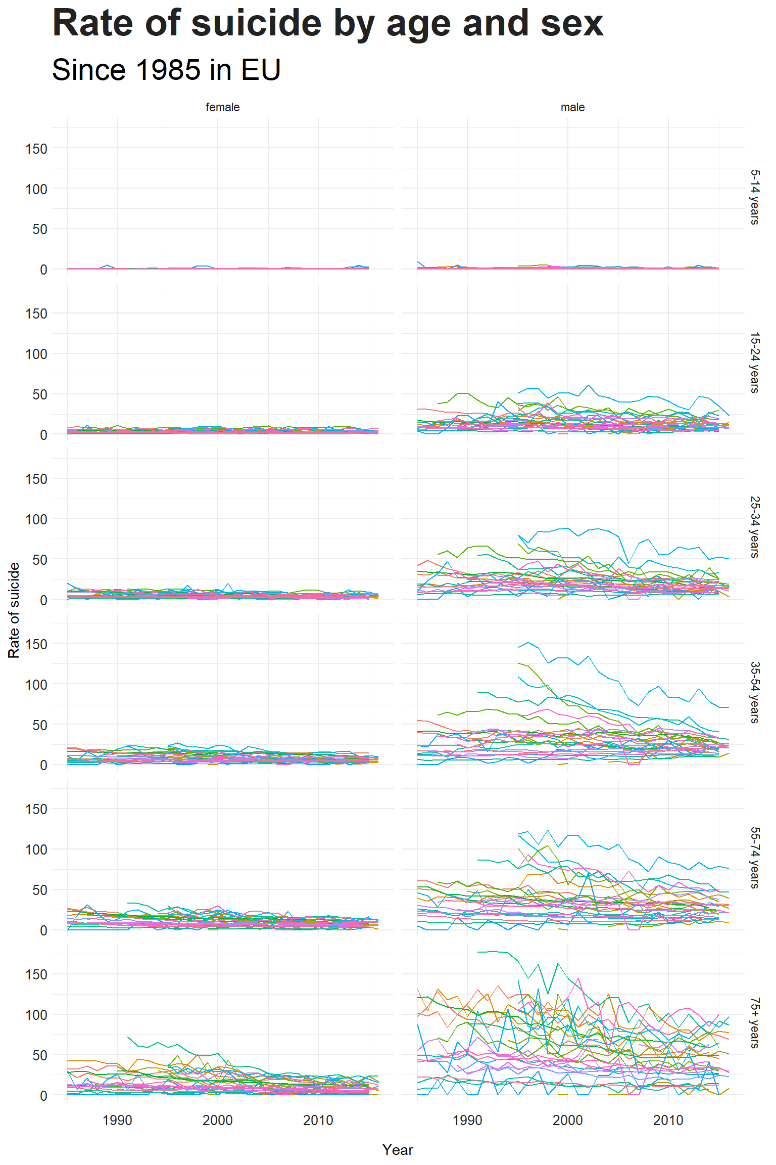
Finland
Number of suicides by sex
data %>% filter(country == "Finland") %>%
  filter(!is.na(suicides_no)) %>%
  ggplot() + geom_point(aes(year, suicides_no, color = fct_reorder2(age, year, suicides_no))) +
  geom_line(aes(year, suicides_no, colour = age)) + facet_wrap(~sex) +
  scale_color_discrete(name = "Age group") +
  labs(title = "Number of suicides by sex", subtitle = "in Finland",
       x = "Year", y = "Number of suicides")
Rate of suicides by sex
data %>% filter(country == "Finland") %>%
  filter(!is.na(suicides_no)) %>%
  ggplot() + geom_point(aes(year, suicides_rate, color = fct_reorder2(age, year, suicides_rate))) +
  geom_line(aes(year, suicides_rate, colour = age)) + facet_wrap(~sex)+
  scale_color_discrete(name = "Age group") +
  labs(title = "Rate of suicides by sex", subtitle = "in Finland",
       x = "Year", y = "Rate of suicides")
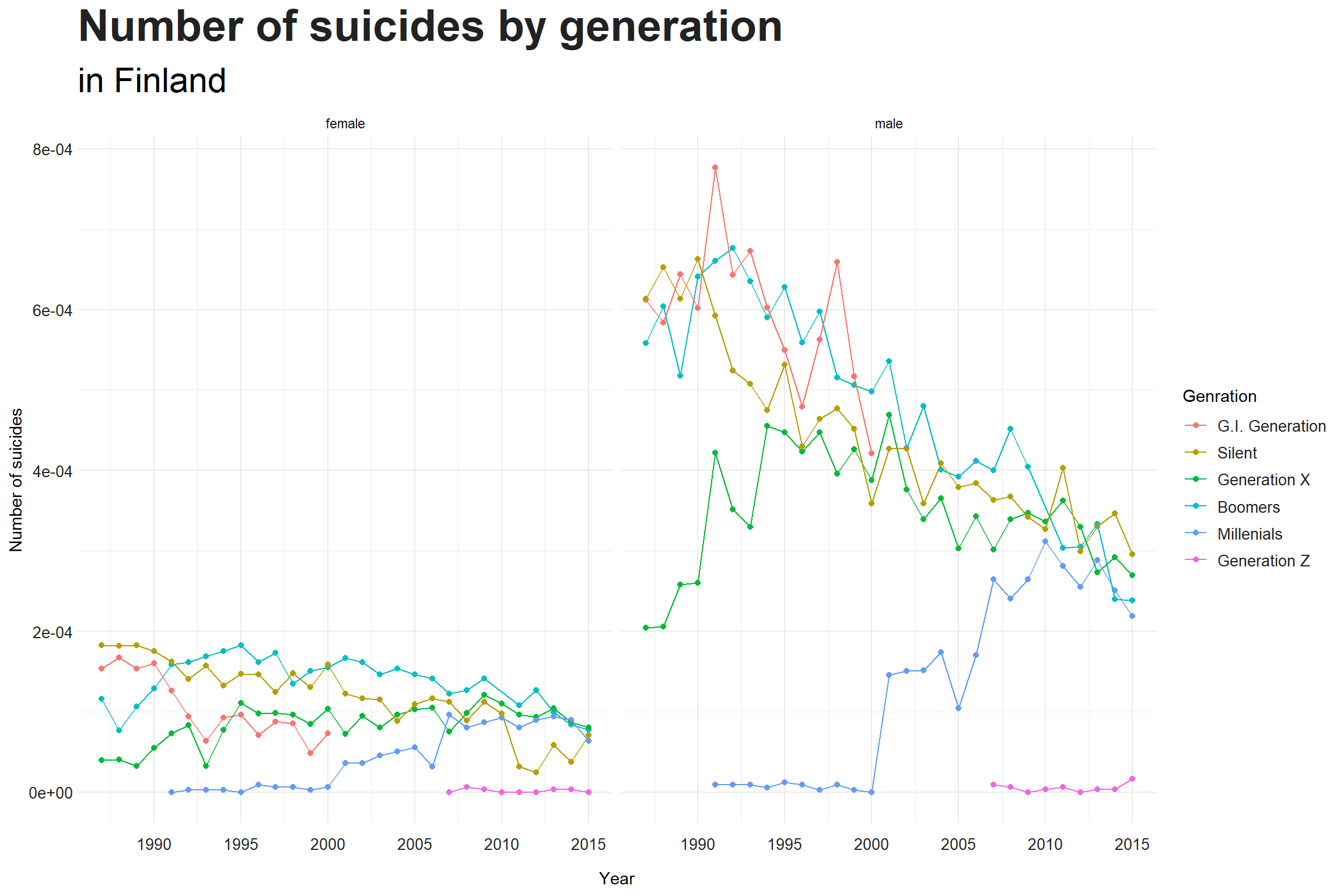
Rate of suicides by generation
data %>% filter(country == "Finland") %>%
  filter(!is.na(suicides_no)) %>% group_by(generation, sex, year) %>%
  summarise(suicides_rate = sum(suicides_no)/sum(population)) %>%
  ggplot() + geom_point(aes(year, suicides_rate, color = fct_reorder2(generation, year, suicides_rate))) +
  geom_line(aes(year, suicides_rate, colour = generation)) + facet_wrap(~sex)+
  scale_color_discrete(name = "Genration") +
  labs(title = "Number of suicides by generation", subtitle = "in Finland",
       x = "Year", y = "Number of suicides")