Table of contents
- Load libraries
- Check data
- Load data
- Preprocess
- Remove outliers
- Aggregate data and add proxy variable
- Event frequency
- Correlation plot
- Cross-correlation
- Time-series plot
- Seasonal pattern based on Event
- Diurnal pattern based on Event
- Check normality assumptions of all parameters for each Event category
- Kruskal-Wallis test
- PCA
- K-nearest neighbor
Intro
One of the major uncertainties in predicting the Earth’s climate are the atmospheric aerosol particles. Being highly variable in space and time, aerosols are very difficult to quantify exactly. This leads to uncertainties in understanding the radiative balance in the atmosphere and predicting precipitation. While primary emissions are huge sources of aerosols particles, New Particle Formation (NPF) is one of the major sources of increase in the particle number in the atmosphere and are seen to occur in diverse atmospheric conditions.
This is the analyses that I made together with Steven Job Thomas. Full report can be found in the beginning by clicking the PDF button, also full code and be found at my github page (also in the beginning of this page).
Load libraries
import pandas as pd
import numpy as np
import matplotlib.pyplot as plt
import matplotlib.dates
import seaborn as sns
Load data
df_raw = pd.read_csv('fulldata.csv', parse_dates = ['Time'])
df_raw.columns = [x if x == "Time" else x[9:] for x in df_raw.columns] # Remove unnecessary part in default column names
df_raw.rename(columns = {'NOx168' : 'NOx', 'O3168' : 'O3', 'RHIRGA168' : 'Rel_Hum', 'O3168': 'Ozone', 'T168' : 'Temp', 'SO2168' : 'SO2'}, inplace = True)
event = pd.read_csv('Event_classification_2004-2014.csv') # Load event data
event['Time'] = pd.to_datetime(event.Date, format = "%d-%b-%Y")
event.drop('Date', axis = 1, inplace = True)

condense_raw = pd.read_csv('CS_2004_2014.csv') # Load condensation sink data
condense_raw['Time'] = pd.to_datetime(condense_raw.times, format = "%d-%b-%Y %H:%M:%S")
condense_raw.drop('times', axis = 1, inplace = True)
condense_raw.rename(columns = {'Condensation_sink': 'CS_sink'}, inplace = True)
Get data from 2008 & 2009
condense_raw = condense_raw[(condense_raw.Time >= pd.Timestamp(2008,1,1)) & (condense_raw.Time < pd.Timestamp(2010,1,1))]
event = event[(event.Time >= pd.Timestamp(2008,1,1)) & (event.Time < pd.Timestamp(2010,1,1))]
condense_raw.reset_index(drop = True, inplace = True)
event.reset_index(drop = True, inplace = True)
# Make a dictionary of variable's names with correct unit.
# Each time a variable is plotted, the correct unit will be extract from this dictionary for labelling
unit = {'CS_sink' : '$s^{-1}$' , 'Rel_Hum' : '%', 'Temp' : '$^\circ C$', 'Ozone' : 'ppb',
       'NOx' : 'ppb', 'SO2' : 'ppb','UV_B' : '$W m^{-2}$', 'H2SO4' : '$cm^{-3}$'}
Check data
Parameters data
print(df_raw.head())
                 Time   NOx  Ozone  Rel_Hum   SO2  Temp    UV_B
0 2008-01-01 00:00:00   NaN    NaN      NaN   NaN -1.79 -0.0003
1 2008-01-01 00:01:00   NaN    NaN      NaN   NaN -1.81  0.0002
2 2008-01-01 00:02:00   NaN    NaN      NaN   NaN -1.80  0.0002
3 2008-01-01 00:03:00  0.57  26.57    85.59 -0.02 -1.84  0.0002
4 2008-01-01 00:04:00   NaN    NaN      NaN   NaN -1.84  0.0006
Overall statistics
print(df_raw.describe())
                 NOx          Ozone        Rel_Hum            SO2  \
count  171339.000000  171201.000000  164762.000000  171681.000000
mean        1.235275      29.356992      76.981689       0.188140
std         1.593818      10.731424      18.947285       0.381855
min        -0.220000      -0.930000      16.330000      -0.220000
25%         0.290000      21.730000      64.870000       0.030000
50%         0.670000      28.810000      84.560000       0.090000
75%         1.610000      36.170000      92.070000       0.210000
max        57.450000      82.590000     105.650000      36.420000

               Temp          UV_B
count  1.039150e+06  1.045704e+06
mean   4.489560e+00  2.476934e-01
std    8.450221e+00  4.978083e-01
min   -2.005000e+01 -6.100000e-03
25%   -1.550000e+00  0.000000e+00
50%    3.650000e+00  6.100000e-03
75%    1.148000e+01  2.215000e-01
max    2.789000e+01  3.216400e+00
Check NA values
# There are plenty of missing values,
# significant difference in number of missing values is from the difference in sampling frequency
df_raw.isna().sum()
Time            0
NOx        881301
Ozone      881439
Rel_Hum    887878
SO2        880959
Temp        13490
UV_B         6936
dtype: int64
Event data
First glance
print(event.head())
   Type Ia  Type Ib  Type II  Type Apple  Type Bump  Type Rain  \
0        0        0        0           0          0          0
1        0        0        0           0          0          0
2        0        0        0           0          0          0
3        0        0        0           0          0          0
4        0        0        0           0          0          0

   Type Featureless  Nonevent  Undefined       Time
0                 0         1          0 2008-01-01
1                 0         0          1 2008-01-02
2                 0         0          0 2008-01-03
3                 0         0          1 2008-01-04
4                 0         1          0 2008-01-05
General statistics
print(event.describe())
          Type Ia     Type Ib     Type II  Type Apple  Type Bump  Type Rain  \
count  731.000000  731.000000  731.000000       731.0      731.0      731.0
mean     0.004104    0.047880    0.151847         0.0        0.0        0.0
std      0.063974    0.213658    0.359118         0.0        0.0        0.0
min      0.000000    0.000000    0.000000         0.0        0.0        0.0
25%      0.000000    0.000000    0.000000         0.0        0.0        0.0
50%      0.000000    0.000000    0.000000         0.0        0.0        0.0
75%      0.000000    0.000000    0.000000         0.0        0.0        0.0
max      1.000000    1.000000    1.000000         0.0        0.0        0.0

       Type Featureless    Nonevent   Undefined
count             731.0  731.000000  731.000000
mean                0.0    0.313269    0.454172
std                 0.0    0.464141    0.498236
min                 0.0    0.000000    0.000000
25%                 0.0    0.000000    0.000000
50%                 0.0    0.000000    0.000000
75%                 0.0    1.000000    1.000000
max                 0.0    1.000000    1.000000
Frequency of each event in the period 2008-2009
event.sum(axis = 0) # Those type never occurred in this period will be removed
Type Ia               3
Type Ib              35
Type II             111
Type Apple            0
Type Bump             0
Type Rain             0
Type Featureless      0
Nonevent            229
Undefined           332
dtype: int64
Check NA values
event.isna().sum()
Type Ia             0
Type Ib             0
Type II             0
Type Apple          0
Type Bump           0
Type Rain           0
Type Featureless    0
Nonevent            0
Undefined           0
Time                0
dtype: int64
Let’s check whether each event is marked only as 1 and 0 or if there is any hidden value
# Sometimes, in old data design, missing values are marked as an arbitrary number like 99, just double check
for col in event.iloc[:,:-1]:
    print(col, event[col].unique())
Type Ia [0 1]
Type Ib [0 1]
Type II [0 1]
Type Apple [0]
Type Bump [0]
Type Rain [0]
Type Featureless [0]
Nonevent [1 0]
Undefined [0 1]
Check if each day, there is only one event
event.sum(axis = 1).unique()
# To check if there is more than one event in a day or data input mistake which mark 'event' and 'nonevent' on the same day
array([1, 0], dtype=int64)
Condense
First glance
print(condense_raw.head())
    CS_sink                Time
0  0.001787 2008-01-01 00:09:45
1  0.001710 2008-01-01 00:19:45
2  0.001514 2008-01-01 00:29:46
3  0.001527 2008-01-01 00:39:45
4  0.001554 2008-01-01 00:49:46
General statistics
print(condense_raw.describe())
             CS_sink
count  102540.000000
mean        0.003777
std         0.003240
min         0.000006
25%         0.001818
50%         0.003016
75%         0.004813
max         0.325251
Check NA values
condense_raw.isna().sum()
CS_sink    1158
Time          0
dtype: int64
Preprocess
Event data
Let’s drop Type Apple, Type Bump, Type Rain and Type Featureless due to no data
event.drop(['Type Apple', 'Type Rain', 'Type Bump', 'Type Featureless'], axis = 1, inplace = True)
New variabable that combines all events and then remove all those event it replaces
event['Event'] = event['Type Ia'] + event['Type Ib'] + event['Type II']
event.drop(['Type Ia', 'Type Ib', 'Type II'], axis = 1, inplace = True)
Replace Event, Nonevent, and Undefined columns by Event_category column
condition = [event.Event == 1, event.Nonevent == 1]
choice = ['Event', 'Nonevent']
event['Event_category'] = np.select(condition, choice, default = 'Undefined')
event.drop(['Nonevent', 'Event', 'Undefined'], axis = 1, inplace = True)
Remove outlier for condense and parameters df
Time-series of each parameter
fig, axe = plt.subplots(df_raw.shape[1] - 1,1, figsize = (15, 30))
axe = axe.flatten()
for i in range(1, df_raw.shape[1]):
    axe[i-1].scatter(df_raw.Time, df_raw.iloc[:,i])
    axe[i-1].set_title(df_raw.columns[i])
    axe[i-1].set_ylabel(unit.get(df_raw.columns[i]))
    axe[i-1].xaxis.set_major_locator(matplotlib.dates.MonthLocator(bymonth=12, bymonthday=1, interval=1, tz=None))

fig.subplots_adjust(left=None, bottom=None, right=None, top=None, wspace=None, hspace=0.5)
C:\Users\VIET\Anaconda3\lib\site-packages\pandas\plotting\_matplotlib\converter.py:103: FutureWarning: Using an implicitly registered datetime converter for a matplotlib plotting method. The converter was registered by pandas on import. Future versions of pandas will require you to explicitly register matplotlib converters.

To register the converters:
    >>> from pandas.plotting import register_matplotlib_converters
    >>> register_matplotlib_converters()
  warnings.warn(msg, FutureWarning)

df_raw.boxplot(figsize = (15, 7))
<matplotlib.axes._subplots.AxesSubplot at 0x1b4ddcf1a20>

Detecting outlier using boxplot for the raw time-series of two years is not ideal because:
Time-series are usually not stationary
If the values only peak during a short time of every year (for example during the last week of every winter), then only a small set of data have such a high values (because there are 53 weeks in a year). As a result, the boxplot will consider those as outlier.
Instead, detecting outlier based on the distribution of the differences between two consecutive observations is a better idea. We wil make a function to remove outlier by first compute the distribution of diffences between two consecutive values. Then those differences that have $ \left | Zscore \right |$ larger than 1.96 (corresponding to within 95% of the distribution) will be considered as outlier. In simple words, the fluctuation between consecutive values will be removed (put as NaN) if they are too large in their distribution.
# Remove outlier based on quantile
#def remove_outlier_quantile(dataframe, quantile = 0.95, timecolumn = 'Time'):
#    data = dataframe.copy(deep = True)
#    for col in data:
#        if col not in [timecolumn]:
#            column_nona = data.loc[~data[col].isna(), col]
#            delta = column_nona - column_nona.shift(1)
#            q = delta.quantile(quantile)
#            idx = delta[delta > q].index
#            data.loc[idx, col] = np.NaN
#    return data
# Remove outlier based on zscore
def remove_outlier(dataframe, zscore = 1.96, timecolumn = 'Time'):
    from scipy import stats
    data = dataframe.copy(deep = True)
    for col in data:
        if col not in [timecolumn]:
            column_nona = data.loc[~data[col].isna(), col]
            delta = column_nona - column_nona.shift(1)
            delta.iloc[0] = np.nanmean(delta) # To include first value of the time series
            abs_zscore = np.abs(stats.zscore(delta))
            idx = delta[abs_zscore > zscore].index
            data.loc[idx, col] = np.NaN
    return data
Remove outliers
df_processed = remove_outlier(df_raw)

condense_processed = remove_outlier(condense_raw)
fig, axe = plt.subplots(df_raw.shape[1] + 1,2, figsize = (15, 30), gridspec_kw={"height_ratios":np.append(0.005, np.repeat(1,df_raw.shape[1]))})

# Make titles for each column of plot
axe[0,0].axis('off')
axe[0,0].set_title('Removed ouliers data', fontweight='bold', fontsize = 20)
axe[0,1].axis('off')
axe[0,1].set_title('Raw data', fontweight='bold', fontsize = 20)

# Plot
for i in range(1, df_raw.shape[1]):
    axe[i, 0].scatter(df_processed.Time, df_processed.iloc[:,i])
    axe[i, 0].set_title(df_processed.columns[i])
    axe[i, 0].set_ylabel(unit.get(df_processed.columns[i]))
    axe[i, 0].xaxis.set_major_locator(matplotlib.dates.MonthLocator(bymonth=12, bymonthday=1, interval=1, tz=None))
    axe[i, 1].scatter(df_raw.Time, df_raw.iloc[:,i])
    axe[i, 1].set_title(df_raw.columns[i])
    axe[i, 1].set_ylabel(unit.get(df_raw.columns[i]))
    axe[i, 1].xaxis.set_major_locator(matplotlib.dates.MonthLocator(bymonth=12, bymonthday=1, interval=1, tz=None))

axe[df_raw.shape[1] , 0].scatter(condense_processed.Time, condense_processed.CS_sink)
axe[df_raw.shape[1] , 0].set_title('CS_sink')
axe[df_raw.shape[1] , 0].set_ylabel(unit.get('CS_sink'))
axe[df_raw.shape[1] , 0].xaxis.set_major_locator(matplotlib.dates.MonthLocator(bymonth=12, bymonthday=1, interval=1, tz=None))
axe[df_raw.shape[1] , 1].scatter(condense_raw.Time, condense_raw.CS_sink)
axe[df_raw.shape[1] , 1].set_title('CS_sink')
axe[df_raw.shape[1] , 1].set_ylabel(unit.get('CS_sink'))
axe[df_raw.shape[1] , 1].xaxis.set_major_locator(matplotlib.dates.MonthLocator(bymonth=12, bymonthday=1, interval=1, tz=None))

fig.subplots_adjust(left=None, bottom=0.1, right=None, top=None, wspace=None, hspace=0.5)

Aggregate data
Calculate hourly data
# Aggregate data by hour and take the mean of all observation within each hour
condense_hourly = condense_processed.groupby([condense_processed["Time"].dt.date,condense_processed["Time"].dt.hour]).mean()
df_hourly = df_processed.groupby([df_processed["Time"].dt.date,df_processed["Time"].dt.hour]).mean()
# Join data together
combined_hourly = condense_hourly.join(df_hourly)
combined_hourly.index.rename(['Time', 'Hour'], inplace = True)
# Join with event data set
event = event.set_index('Time')
combined_hourly =event.join(combined_hourly)
Calculate daily data
# Aggregate data by date and take the mean of all observation within each date
condense_daily = condense_processed.groupby([condense_processed["Time"].dt.date]).mean()
df_daily = df_processed.groupby([df_processed["Time"].dt.date]).mean()
# Join data
combined_daily = event.join(condense_daily).join(df_daily)
Add proxy
$[H_2SO4]{proxy} = k \cdot \frac{[SO_2][UVB]}{CS}$
combined_daily['H2SO4'] = combined_daily['SO2'] * combined_daily['UV_B'] * 9.9e-7 / combined_daily['CS_sink'] * 2.62e-6 / 64 * 6.023e23 / 1e6
combined_hourly['H2SO4'] = combined_hourly['SO2'] * combined_hourly['UV_B'] * 9.9e-7 / combined_hourly['CS_sink'] * 2.62e-6 / 64 * 6.023e23 / 1e6
Analysis
Event frequency
from matplotlib import colors
# Make dataframe for the calendar plot
value_to_int = {j:i+1 for i,j in enumerate(pd.unique(event.values.ravel()))}
event_cal = event.replace(value_to_int)
cal = {'2008': event_cal[event_cal.index.year == 2008], '2009': event_cal[event_cal.index.year == 2009]}
# Define Ticks
DAYS = ['Sun', 'Mon', 'Tues', 'Wed', 'Thurs', 'Fri', 'Sat']
MONTHS = ['Jan', 'Feb', 'Mar', 'Apr', 'May', 'June', 'July', 'Aug', 'Sept', 'Oct', 'Nov', 'Dec']

fig, ax = plt.subplots(2, 1, figsize = (20,6))
for i, val in enumerate(['2008', '2009']):
    start = cal.get(val).index.min()
    end = cal.get(val).index.max()
    start_sun = start - np.timedelta64((start.dayofweek + 1) % 7, 'D')
    end_sun =  end + np.timedelta64(7 - end.dayofweek -1, 'D')

    num_weeks = (end_sun - start_sun).days // 7
    heatmap = np.zeros((7, num_weeks))
    ticks = {}
    y = np.arange(8) - 0.5
    x = np.arange(num_weeks + 1) - 0.5
    for week in range(num_weeks):
        for day in range(7):
            date = start_sun + np.timedelta64(7 * week + day, 'D')
            if date.day == 1:
                ticks[week] = MONTHS[date.month - 1]
            if date.dayofyear == 1:
                ticks[week] += f'\n{date.year}'
            if start <= date < end:
                heatmap[day, week] = cal.get(val).loc[date, 'Event_category']

    cmap = colors.ListedColormap(['gray', 'tab:blue', 'whitesmoke', 'tab:orange'])
    mesh = ax[i].pcolormesh(x, y, heatmap, cmap = cmap, edgecolors = 'grey')

    ax[i].invert_yaxis()

    # Set the ticks.
    ax[i].set_xticks(list(ticks.keys()))
    ax[i].set_xticklabels(list(ticks.values()))
    ax[i].set_yticks(np.arange(7))
    ax[i].set_yticklabels(DAYS)
    ax[i].set_ylim(6.5,-0.5)
    ax[i].set_aspect('equal')
    ax[i].set_title(val, fontsize = 15)
# Add color bar at the bottom
cbar_ax = fig.add_axes([0.25, -0.10, 0.5, 0.05])
fig.colorbar(mesh, orientation="horizontal", pad=0.2, cax = cbar_ax)
n = len(value_to_int) +1
colorbar = ax[1].collections[0].colorbar
r = colorbar.vmax - colorbar.vmin
colorbar.set_ticks([colorbar.vmin + r / n * (0.5 + i) for i in range(n)])
colorbar.set_ticklabels(['Outofbound'] + list(value_to_int.keys()))
fig.suptitle('Frequency of events', fontweight = 'bold', fontsize = 25)
fig.subplots_adjust(hspace = 0.5)

Correlation plot
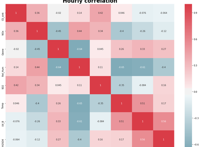
fig, ax = plt.subplots(figsize = (17,12))
sns.heatmap(combined_hourly.corr(), cmap = cmap, center=0.00, ax = ax, annot = True)
ax.set_ylim(combined_hourly.shape[1]-1,0)
ax.set_title('Hourly correlation', weight = "bold", fontsize=24)

fig, ax = plt.subplots(1, 2, figsize = (20,8))
sns.heatmap(combined_daily[combined_daily.Event_category == 'Event'].corr(), cmap = cmap, center=0.00, ax = ax[0], annot = True, cbar = False)
ax[0].set_ylim(combined_daily.shape[1]-1,0)
ax[0].set_title('Daily correlation on Event day', weight = "bold", fontsize=24)
sns.heatmap(combined_daily[combined_daily.Event_category == 'Nonevent'].corr(), cmap = cmap, center=0.00, ax = ax[1], annot = True, cbar = True)
ax[1].set_ylim(combined_daily.shape[1]-1,0)
ax[1].set_title('Daily correlation on Non-Event day', weight = "bold", fontsize=24)
Text(0.5, 1, 'Daily correlation on Non-Event day')

Cross-correlation
# Make an empty matrix n x n with n is the number of parameters.
cross_correlation = np.zeros((combined_hourly.shape[1] - 1, combined_hourly.shape[1] - 1))
# Loop all values in the matrix and compute the corresponding time-lag
for ii, i in enumerate(combined_hourly.columns[1:]):
    for jj, j in enumerate(combined_hourly.columns[1:]):
        if j != i:
            pair = combined_hourly[[i, j]].dropna(axis = 0)
            c = np.correlate(pair[i], pair[j], mode = 'full')
            icmax = np.argmax(c)
            tlag = -1 * (icmax - len(pair[i]) +1)
            cross_correlation[ii,jj] = tlag
# Plot heatmap of the matrix
fig, ax = plt.subplots(figsize = (17,12))
sns.heatmap(cross_correlation.astype(int), xticklabels = combined_hourly.columns[1:], yticklabels = combined_hourly.columns[1:], ax = ax, annot = True, fmt="d", cmap = cmap)
ax.set_ylim(combined_hourly.shape[1] -1 ,0)
fig.suptitle('Cross correlation between all parameters', fontweight = 'bold', size = 22)
ax.set_title('Value of each cell is time lag (hour)')
Text(0.5, 1, 'Value of each cell is time lag (hour)')

Cross-correlation is a measure of similarity of two time-series as a function of a time-lag applied to one of them. In this result, those pairs of parameters that have time-lag too far away from 0 is probably not similar
Time-series plot
fig, axe = plt.subplots(combined_daily.shape[1]-1, figsize = (15, 30))
for i in range(combined_daily.shape[1]-1):
    axe[i].plot(combined_daily[combined_daily.Event_category == 'Event'].iloc[:,i+1],'.', markersize = 8 ,label = 'Event day')
    axe[i].plot(combined_daily[combined_daily.Event_category == 'Nonevent'].iloc[:,i+1], '.' , markersize = 8,c = 'red', label = 'Nonevent day')
#    axe[i].plot(combined_daily[combined_daily.Event_category == 'Undefined'].iloc[:,i+1], c = 'green', marker = '.', label = 'Undefined day')
    axe[i].set_title(combined_daily.columns[i+1], fontweight = 'bold')
    axe[i].set_ylabel(unit.get(combined_daily.columns[i+1]))
    axe[i].xaxis.set_major_locator(matplotlib.dates.MonthLocator(bymonth=12, bymonthday=1, interval=1, tz=None))
    axe[i].legend()

fig.subplots_adjust(left=None, bottom=None, right=None, top=None, wspace=None, hspace=0.5)

Seasonal pattern based on Event
fig, ax = plt.subplots(combined_daily.shape[1] - 1, figsize = (15, 55))
for i in range(combined_daily.shape[1] - 1):
    sns.boxplot(x = combined_daily.index.month, y = combined_daily.iloc[:,i+1], hue = combined_daily['Event_category'], palette = {'Nonevent' : 'tab:blue', 'Undefined' : 'whitesmoke', 'Event' : 'tab:orange'}, hue_order = ['Event', 'Nonevent', 'Undefined'], ax = ax[i])
    ax[i].set_title(combined_daily.columns[i+1], fontweight = 'bold')
    ax[i].set_xlabel('Month')
    ax[i].set_ylabel(unit.get(combined_daily.columns[i+1]))
    ax[i].set_xticklabels(MONTHS)

fig.subplots_adjust(left=None, bottom=None, right=None, top=None, wspace=None, hspace=0.5)

Diurnal pattern based on Event
WINTER
winter = [12,1,2,3] # Define months of winter
idx = np.in1d(combined_hourly.index.get_level_values('Time').month, winter)
fig, ax = plt.subplots(combined_hourly.shape[1] - 1, figsize = (15, 85))
for i in range(combined_hourly.shape[1] - 1):
    sns.boxplot(x = combined_hourly[idx].index.get_level_values('Hour'), y = combined_hourly[idx].iloc[:,i+1], hue = combined_hourly.loc[idx,'Event_category'], palette = {'Nonevent' : 'tab:blue', 'Undefined' : 'whitesmoke', 'Event' : 'tab:orange'}, hue_order = ['Event', 'Nonevent', 'Undefined'], ax = ax[i])
    ax[i].set_title(combined_daily.columns[i+1] + ' in winter', fontweight = 'bold')
    ax[i].set_ylabel(unit.get(combined_daily.columns[i+1]))
    ax[i].set_xlabel('Hour')

SPRING
spring = [4, 5] # Define months of spring
idx = np.in1d(combined_hourly.index.get_level_values('Time').month, spring)
fig, ax = plt.subplots(combined_hourly.shape[1] - 1, figsize = (15, 85))
for i in range(combined_hourly.shape[1] - 1):
    sns.boxplot(x = combined_hourly[idx].index.get_level_values('Hour'), y = combined_hourly[idx].iloc[:,i+1], hue = combined_hourly.loc[idx,'Event_category'], palette = {'Nonevent' : 'tab:blue', 'Undefined' : 'whitesmoke', 'Event' : 'tab:orange'}, hue_order = ['Event', 'Nonevent', 'Undefined'], ax = ax[i])
    ax[i].set_title(combined_daily.columns[i+1] + ' in spring', fontweight = 'bold')
    ax[i].set_xlabel('Hour')
    ax[i].set_ylabel(unit.get(combined_daily.columns[i+1]))

SUMMER
summer = [6,7,8] # # Define months of summer
idx = np.in1d(combined_hourly.index.get_level_values('Time').month, summer)
fig, ax = plt.subplots(combined_hourly.shape[1] - 1, figsize = (15, 85))
for i in range(combined_hourly.shape[1] - 1):
    sns.boxplot(x = combined_hourly[idx].index.get_level_values('Hour'), y = combined_hourly[idx].iloc[:,i+1], hue = combined_hourly.loc[idx,'Event_category'], palette = {'Nonevent' : 'tab:blue', 'Undefined' : 'whitesmoke', 'Event' : 'tab:orange'}, hue_order = ['Event', 'Nonevent', 'Undefined'], ax = ax[i])
    ax[i].set_title(combined_daily.columns[i+1] + ' in summer', fontweight = 'bold')
    ax[i].set_xlabel('Hour')
    ax[i].set_ylabel(unit.get(combined_daily.columns[i+1]))

AUTUMN
autumn = [9,10,11] # # Define months of autumn
idx = np.in1d(combined_hourly.index.get_level_values('Time').month, autumn)
fig, ax = plt.subplots(combined_hourly.shape[1] - 1, figsize = (15, 85))
for i in range(combined_hourly.shape[1] - 1):
    sns.boxplot(x = combined_hourly[idx].index.get_level_values('Hour'), y = combined_hourly[idx].iloc[:,i+1], hue = combined_hourly.loc[idx,'Event_category'], palette = {'Nonevent' : 'tab:blue', 'Undefined' : 'whitesmoke', 'Event' : 'tab:orange'}, hue_order = ['Event', 'Nonevent', 'Undefined'], ax = ax[i])
    ax[i].set_title(combined_daily.columns[i+1] + ' in autumn', fontweight = 'bold')
    ax[i].set_xlabel('Hour')
    ax[i].set_ylabel(unit.get(combined_daily.columns[i+1]))

Check normality assumptions of all parameters for each Event category
fig, ax = plt.subplots(4,2, figsize = (15,10))
ax = ax.flatten()
for i, ax in enumerate(ax):
    ax.hist(combined_daily[combined_daily['Event_category'] == 'Nonevent'].iloc[:,i+1])
    ax.set_title(combined_daily.columns[i+1])
    ax.set_ylabel(unit.get(combined_daily.columns[i+1]))


fig.subplots_adjust(hspace = 0.5)
fig.suptitle('Check normality of all parameters for Nonevent', fontweight = 'bold', size = 16)
C:\Users\VIET\Anaconda3\lib\site-packages\numpy\lib\histograms.py:824: RuntimeWarning: invalid value encountered in greater_equal
  keep = (tmp_a >= first_edge)
C:\Users\VIET\Anaconda3\lib\site-packages\numpy\lib\histograms.py:825: RuntimeWarning: invalid value encountered in less_equal
  keep &= (tmp_a <= last_edge)


Text(0.5, 0.98, 'Check normality of all parameters for Nonevent')

fig, ax = plt.subplots(4,2, figsize = (15,10))
ax = ax.flatten()
for i, ax in enumerate(ax):
    ax.hist(combined_daily[combined_daily['Event_category'] == 'Event'].iloc[:,i+1])
    ax.set_title(combined_daily.columns[i+1])
    ax.set_ylabel(unit.get(combined_daily.columns[i+1]))
fig.subplots_adjust(hspace = 0.5)
fig.suptitle('Check normality of all parameters for Event', fontweight = 'bold', size = 16)
Text(0.5, 0.98, 'Check normality of all parameters for Event')

They are not normally distributed, need to use Non-parametric tests
Kruskal-Wallis test
Test if values for each parameters are significant different from each Event category (Nonevent, Event and Undefined)
from scipy.stats import kruskal
Event = combined_daily[combined_daily.Event_category == 'Event']
Nonevent = combined_daily[combined_daily.Event_category == 'Nonevent']
Undefined = combined_daily[combined_daily.Event_category == 'Undefined']
for i, col in enumerate(combined_daily.columns[1:]):
    stat, p = kruskal(Event[col].dropna(axis = 0).values, Nonevent[col].dropna(axis = 0).values, Undefined[col].dropna(axis = 0).values)
    print('\033[1m' + col + '\033[0m' ) # Bold print--pretty cool
    print(f'Statistics :{stat}, p value = {p}')
    if p < 0.05:
        print("Reject NULL hypothesis - Significant differences exist between groups.")
    if p > 0.05:
        print("Accept NULL hypothesis - No significant difference between groups.")
    print('-' * 100 + '\n')
[1mCS_sink[0m
Statistics :100.17401361194061, p value = 1.7680287756421552e-22
Reject NULL hypothesis - Significant differences exist between groups.
----------------------------------------------------------------------------------------------------
[1mNOx[0m
Statistics :83.0958197351556, p value = 9.035912357580163e-19
Reject NULL hypothesis - Significant differences exist between groups.
----------------------------------------------------------------------------------------------------
[1mOzone[0m
Statistics :99.62119111341462, p value = 2.330951350458591e-22
Reject NULL hypothesis - Significant differences exist between groups.
----------------------------------------------------------------------------------------------------
[1mRel_Hum[0m
Statistics :174.6423531207879, p value = 1.1936991002620061e-38
Reject NULL hypothesis - Significant differences exist between groups.
----------------------------------------------------------------------------------------------------
[1mSO2[0m
Statistics :12.428610331510804, p value = 0.002000605957111047
Reject NULL hypothesis - Significant differences exist between groups.
----------------------------------------------------------------------------------------------------
[1mTemp[0m
Statistics :25.212777518750045, p value = 3.3505409103846863e-06
Reject NULL hypothesis - Significant differences exist between groups.
----------------------------------------------------------------------------------------------------
[1mUV_B[0m
Statistics :109.15560638778243, p value = 1.9822628347049566e-24
Reject NULL hypothesis - Significant differences exist between groups.
----------------------------------------------------------------------------------------------------
[1mH2SO4[0m
Statistics :192.6750391648502, p value = 1.449261799967792e-42
Reject NULL hypothesis - Significant differences exist between groups.
----------------------------------------------------------------------------------------------------
Event day data on 2009 vs 2008 in late spring and early summer
period = [4,5,6]

period_data = combined_daily[np.in1d(combined_daily.index.month, period)] # Get data with month 4,5,6
y2008 = period_data[period_data.index.year == 2008] # Get 2008
y2009 = period_data[period_data.index.year == 2009] # Get 2008
y2008_event = y2008[y2008.Event_category == 'Event'] # Get only Event data
y2009_event = y2009[y2009.Event_category == 'Event'] # Get only Event data


for i, col in enumerate(combined_daily.columns[1:]):
    stat, p = kruskal(y2008_event[col].dropna(axis = 0).values, y2009_event[col].dropna(axis = 0).values)
    print('\033[1m' + col + '\033[0m' ) # Bold print--pretty cool
    print(f'Statistics :{stat}, p value = {p}')
    if p < 0.05:
        print("Reject NULL hypothesis - Significant differences exist between groups.")
    if p > 0.05:
        print("Accept NULL hypothesis - No significant difference between groups.")
    print('-' * 100 + '\n')
[1mCS_sink[0m
Statistics :5.354570135746627, p value = 0.020668028699104363
Reject NULL hypothesis - Significant differences exist between groups.
----------------------------------------------------------------------------------------------------
[1mNOx[0m
Statistics :0.20923076923077133, p value = 0.647370988319673
Accept NULL hypothesis - No significant difference between groups.
----------------------------------------------------------------------------------------------------
[1mOzone[0m
Statistics :0.004524886877845802, p value = 0.946368925124135
Accept NULL hypothesis - No significant difference between groups.
----------------------------------------------------------------------------------------------------
[1mRel_Hum[0m
Statistics :0.06533936651584327, p value = 0.79824762378497
Accept NULL hypothesis - No significant difference between groups.
----------------------------------------------------------------------------------------------------
[1mSO2[0m
Statistics :0.06533936651584327, p value = 0.79824762378497
Accept NULL hypothesis - No significant difference between groups.
----------------------------------------------------------------------------------------------------
[1mTemp[0m
Statistics :1.0454298642533786, p value = 0.3065619830552169
Accept NULL hypothesis - No significant difference between groups.
----------------------------------------------------------------------------------------------------
[1mUV_B[0m
Statistics :1.5992760180995447, p value = 0.20600583969615863
Accept NULL hypothesis - No significant difference between groups.
----------------------------------------------------------------------------------------------------
[1mH2SO4[0m
Statistics :3.5475113122172104, p value = 0.059634830090459216
Accept NULL hypothesis - No significant difference between groups.
----------------------------------------------------------------------------------------------------
Significant differences found in all parameters except CS_sink between 2008 and 2009 events during April, May and June
Boxplot comparing value of CS_sink in event days in 2008 and 2009
fig, ax = plt.subplots(2,1, figsize = (20,7))
sns.boxplot(y2008_event['CS_sink'], ax = ax[0])
ax[0].set_title('2008')
ax[0].set_xlim(0,0.006)
ax[0].set_xlabel(unit.get('CS_sink'))
sns.boxplot(y2009_event['CS_sink'], ax = ax[1])
ax[1].set_title('2009')
ax[1].set_xlim(0,0.006)
ax[1].set_xlabel(unit.get('CS_sink'))

fig.subplots_adjust(hspace = 0.5)
fig.suptitle('CS_sink on event days in 2008 and 2009 April, May and June', fontweight = 'bold', size = 15)
Text(0.5, 0.98, 'CS_sink on event days in 2008 and 2009 April, May and June')

PCA
This PCA method ignore temporal variance of the data. Each observation is treated as independent from each other
# Standardize data
from sklearn.preprocessing import StandardScaler
x = combined_daily.dropna(axis = 0).drop('Event_category', axis = 1).values
y = combined_daily.dropna(axis = 0)['Event_category'].values
x = StandardScaler().fit_transform(x)

# PCA
from sklearn.decomposition import PCA
pca = PCA(0.95)
pca_result = pca.fit_transform(x)
print(f'Number of components: {pca.explained_variance_ratio_.shape[0]}')
print(f'Explained variance of each components: {pca.explained_variance_ratio_}')
Number of components: 6
Explained variance of each components: [0.48555121 0.21419643 0.12958403 0.07393715 0.04262152 0.02679078]
Plot cummulative sum variance explained by each components
fig, ax = plt.subplots()
ax.plot(np.cumsum(pca.explained_variance_ratio_))
ax.set_xticks([0, 1,2,3,4,5])
# ax.set_xlim(0,6)
ax.set_xticklabels(list(np.arange(1,7)))
ax.set_title('Cummulative sum of explained variance by each component', fontweight = 'bold', size = 15)
ax.set_xlabel('Number of components')
ax.set_ylabel('Explained variance')
Text(0, 0.5, 'Explained variance')

Reduce data to only 6 variables. Not impressive at all
Plot data on first two components
# Plot on first two components
fig, ax = plt.subplots(1,1,figsize = (15,8))
ax.set_xlabel('Principal Component 1', fontsize = 15)
ax.set_ylabel('Principal Component 2', fontsize = 15)
ax.set_title('2 component PCA', fontsize = 20)
color = {'Event': 'blue', 'Nonevent' : 'green', 'Undefined' : 'grey'}

for i in ['Undefined', 'Nonevent', 'Event']:
    mask = y == i
    plt.scatter(pca_result[mask, 0], pca_result[mask, 1], label=i, c = color.get(i), alpha = 1)
ax.legend()
print(f'Explained variance of each components{pca.explained_variance_ratio_[:2]}')
Explained variance of each components[0.48555121 0.21419643]

With just two components, PCA is able to separate Event and Nonevent visually :)
K-nearest neighbor
K-nearest neighbor method ignore temporal variance of the data. Each observation is treated as independent from each other
from sklearn.neighbors import KNeighborsClassifier
from sklearn.model_selection import train_test_split
from sklearn.metrics import confusion_matrix
from sklearn.metrics import accuracy_score

# Split to train and test set
X_train, X_test, y_train, y_test = train_test_split(x, y, random_state=1)

# K-nearest neighbor
knn = KNeighborsClassifier(n_neighbors=5, metric='euclidean')
knn.fit(X_train, y_train)
y_pred = knn.predict(X_test)

# Generate confusion matrix to evaluate on test set
classes = np.unique(y)
cm = confusion_matrix(y_test, y_pred, classes)

# Plot the confusion matrix
fig, ax = plt.subplots(figsize = (10, 8))
sns.heatmap(cm, xticklabels = classes, yticklabels = classes,
            annot = True, fmt="d", ax = ax)
ax.set_ylim(3,0)
ax.set_ylabel('True label', size = 10, fontweight = 'bold')
ax.set_xlabel('Predicted label', size = 10, fontweight = 'bold')
ax.set_title(f'Overall accuracy {accuracy_score(y_test, y_pred):.2}', fontweight = 'bold', fontstyle = 'italic')

fig.suptitle('Confusion matrix for K-nearest neighbor algorithm', size = 17, fontweight = 'bold')
Text(0.5, 0.98, 'Confusion matrix for K-nearest neighbor algorithm')

Even though overall accuracy is only 0.61, the algorithm is doing extremely well at not mixing up prediction between Event and Nonevent.
K-fold cross validation
Just to give better estimate of accuracy for new unseen data
# Import KFold class from scikitlearn library
from sklearn.model_selection import KFold

K=5    # number of folds/rounds/splits
kf = KFold(n_splits=K, shuffle=False)
kf = kf.split(x)
kf = list(kf)                 # kf is a list representing the rounds of k-fold CV


train_acc_per_cv_iteration = []
test_acc_per_cv_iteration = []

# for loop over K rounds

for train_indices, test_indices in kf:

    reg = KNeighborsClassifier(n_neighbors=5, metric='euclidean')
    reg = reg.fit(x[train_indices,:], y[train_indices])
    y_pred_train = reg.predict(x[train_indices,:])
    train_acc_per_cv_iteration.append(accuracy_score(y[train_indices], y_pred_train))
    y_pred_val = reg.predict(x[test_indices,:])
    test_acc_per_cv_iteration.append(accuracy_score(y[test_indices], y_pred_val))


acc_train= np.mean(train_acc_per_cv_iteration) # compute the mean of round-wise training acc
acc_val = np.mean(test_acc_per_cv_iteration)   # compute the mean of round-wise validation acc

print("Training accuracy (averaged over 5 folds): ",acc_train)
print("Validation accuracy (averaged over 5 folds):", acc_val)
Training accuracy (averaged over 5 folds):  0.7520565018695471
Validation accuracy (averaged over 5 folds): 0.5205762871988663
The overall accuracy in smaller in cross-validation. It shows that in the first train and test split, we were lucky at getting indices to get the high accuracy in the test set